Excel’s list of functions is one of the most dynamic elements in data analysis. From fancy arithmetic operations to advanced conditional logic, there is a little bit of something for every kind of user out there.

The SUMIFS function is one of the many functions available to users wishing to drive detailed analysis based on conditional logic. If you are familiar with the SUMIF function in Excel, you will find the SUMIFS function is quite similar to its counterpart. Here’s what you need to know about using the SUMIFS function in Excel.

Syntax of a SUMIFS Function

The SUMIFS function in Excel is the culmination of the SUM and IF functions. It sums the values in a cell based on specific criteria. You can create conditions related to dates, numbers, and text. Additionally, feel free to use logical operators to manipulate your conditions and make them more expansive.

To master these logical formulas, you need to know how to use the IFS function, before combining it with any aggregator functions.

Excel has other logical functions, such as COUNTIF, COUNTIFS, SUMIF, MAXIFS, MINIFS, and many others. When working with any of these functions, you must ensure you pass the right syntax within the formulas.

Here’s the syntax of the SUMIFS Function:

        =SUMIFS (sum_range, range1, criteria1, [range2], [criteria2], ...)
    

Where:

• sum_range: The range/column to sum based on your criteria
• range1: Range1 defines the column in which your formula will find the first criteria set
• criteria1: Criteria1 refers to the first condition
• range2: Range2 defines the column in which your formula will find the second criteria set
• criteria2: Criteria2 refers to the second condition

How to Use the SUMIFS Function in Excel

Now that the syntax is out of the way, it is essential to understand the various components of the function and how you can best use it. The SUMIF function has a lot of uses in the data world, but that does not mean the SUMIFS function is far away. You can pass multiple conditions within the SUMIFS formula and take the SUMIF function up a notch.

Data Preparation

Suppose you have a dataset containing information on products sold in an office factory. Some relevant data columns include the order date, category, color, sale price, quantity sold, and total sales. All formulas will be based on the data references included in this sample data.

1. Working With Text Conditions

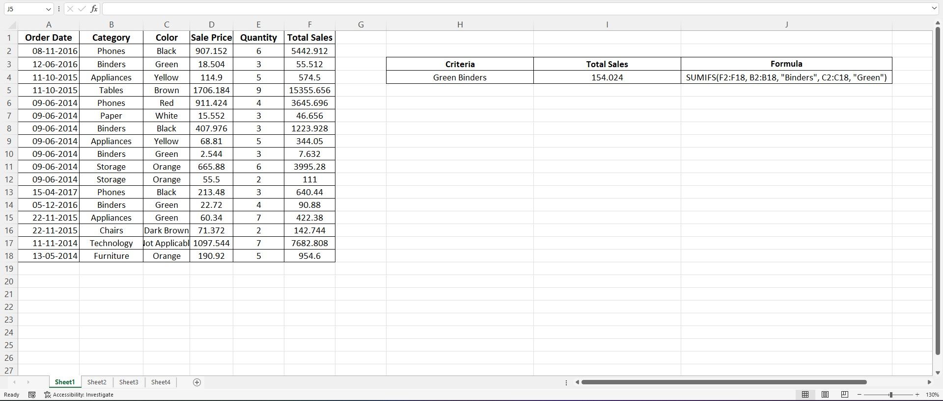
If you want to calculate the total cost of Green Binders from this list, you can use the SUMIFS formula as follows:

        =SUMIFS(F2:F18, B2:B18, "Binders",C2:C18, "Green")
    

First, you must define the column you want to get the totals from; in this case, it is the Total Sales column. Define the column range that has the Binders value (column A). The subsequent part of the formula needs the criteria, Binders.

The first criterion is set; to define the next segment, which is color, you must follow a similar rule. You need to include the column that holds the color details, followed by the color (Green) you want to look for.

Excel calculates the values based on the specified conditions and gives the result 154.024.

2. Working With Numeric Conditions

In the above example, you defined Text conditions (Color = Green and Category = Binders). Now, the next step is to work with numerical conditions. Let's illustrate this with an example:

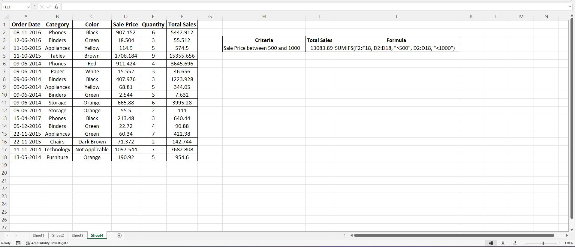
If you want to calculate the total sales for products with a Sale Price between 500 and 1000. Here's how you can construct the formula:

        =SUMIFS(E2:E18, D2:D18, ">500", D2:D18, "<1000")
    

The above formula's first range is the Total Sales column reference. In the next segment, you must define the column for the first criterion, which captures values above 500. In the final part, you must define the final criterion, which captures values below 1000.

The final result is 13083.888.

3. Working With Date Conditions

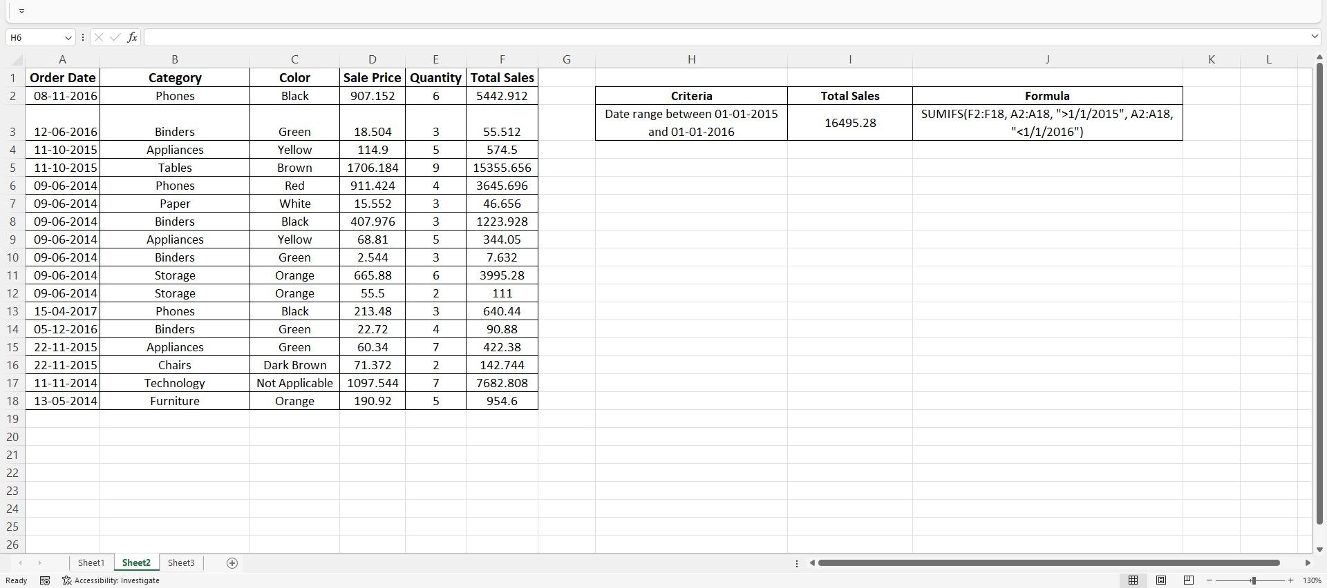
You can use the SUMIFS function to sum values basis date conditions. For example, if you have a set of columns with dates and want to find the total sales during a date range, you can use the formula to derive the result quickly.

        =SUMIFS(F2:F18, A2:A18, ">1/1/2015", A2:A18, "<1/1/2016")
    

Like the other formulas above, you can use dates to manipulate your data and sum the total sales values. The first part of the formula refers to the Total Sales column. In the next segment, you need to define the date ranges. You need to use logical operators to manipulate dates within the SUMIFS formula.

Since the reference includes the dates between 01-01-2015 and 01-01-2016, the result is 16495.28.

4. Using Wildcard Searches

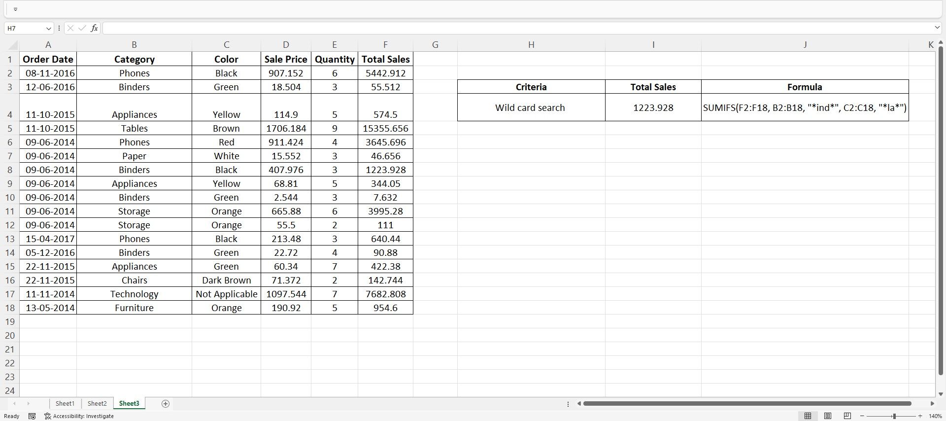
Finally, there is one last method to use with the SUMIFS function. You can aptly combine the wildcard search function with the multi-functional SUMIFS function to find matches based on certain elements. For example, suppose you want to find the sum of values that contain the letters ind within the Category column, and the letters la in the Color column.

Excel's SUMIFS function filters through each specified column and looks for the specified letters. Any matching values are summed up, and the result is displayed. To use the wildcard search, you can either use the * (asterix) sign or the ? (question mark) symbol within your formula.

Here's how you can write the formula:

        =SUMIFS(F2:F18, B2:B18, "*ind*", C2:C18, "*la*")
    

The result is 1223.928.

Using the SUMIFS Function in Excel Efficiently

Despite the widespread use of the SUMIFS function within Excel, many analysts continue to rely on the true potential of this powerful function. There are plenty of ways you can use this multi-faceted function in your regular reporting and analysis.

No matter if you are a freelancer, a shopkeeper, or a data analyst, chances are there will always be a way for you to make the most of this function.