A lot of times, we use sequential numbers to organize large sets of data. Instead of manually typing numbers beside the data, you can simply use the SEQUENCE function to perform this task.
It is an extremely easy function that allows nesting, which means you can get creative with the formula and perform many other complex calculations, saving you a lot of time and frustration.
This article discusses the syntax for this formula and a few examples to help you better understand this formula works. So, read on to master the SEQUENCE function in Google Sheets.
What Is SEQUENCE in Google Sheets?
SEQUENCE is a function that auto-fills cells in Google Sheets depending on the parameters you give in the formula. It works by sequentially counting from where you tell it to into all the cells you specify. Each cell should contain unique values, which will make building certain spreadsheet types easier.
You can find the function by navigating to Insert > Function > Maths. To better understand, let’s dive into the bones of how the function works.
Syntax of SEQUENCE in Google Sheets
The formula for SEQUENCE uses four arguments, three of which are optional. Here’s the formula for SEQUENCE in Google Sheets:
=SEQUENCE(row, column, start, step)
Here is what each of the arguments in this formula represent:
- row: is a required argument that specifies the rows you need to return
- column: This optional argument defines the number of columns you wish to return. If left empty, the array will only have one column.
- start: This is also an optional argument that defines the number to start the sequence with. If left empty, "1" will be used to start the sequence.
- step: This is another optional argument that defines the difference between each number. If left empty, the difference between numbers in the array will be 1.
Examples of the SEQUENCE Function in Google Sheets
Looking at the formula’s syntax gives us a basic idea of using the function. However, looking at the formula in action can further improve your understanding. Here are a few examples of the SEQUENCE formula in Google Sheets to help you master it.
Single Column Sequence
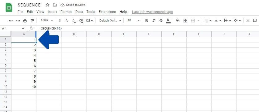
This is the most commonly used application of SEQUENCE in spreadsheets. It generates a vertical list of numbers in a single column. The length of the list is defined by the row argument you use. Here are steps to follow to build a single column sequence:
- Click on the cell where you want to input the formula, A1 in the example.
- Write the beginning of the formula, which is =SEQUENCE(
- Write the number of rows that you wish to create. In this case, we write 10.
- Now, enter the closing bracket to finish the formula.
- Press Enter to execute the formula.
In this instance, the only argument we needed to define was the number of rows in which we wanted to display the numbers.
Single Row Sequence
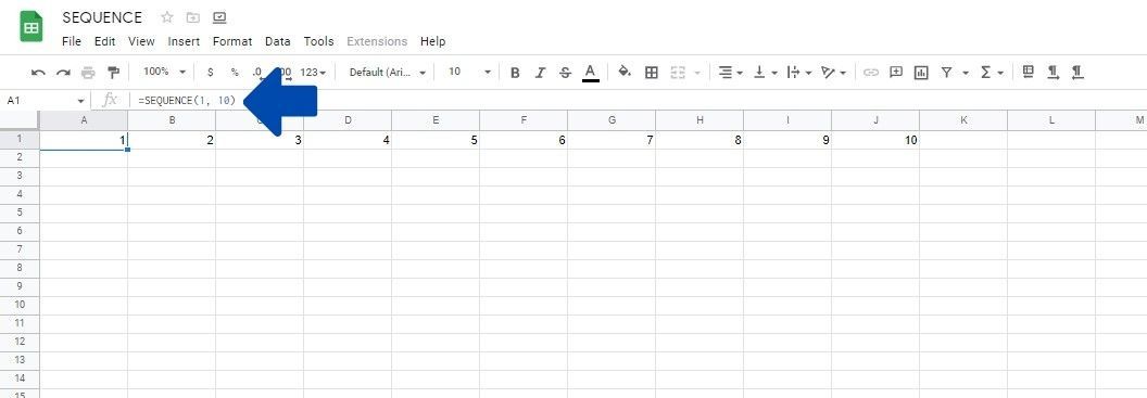
This is also another widespread use case scenario for the SEQUENCE function. It works similarly to the previous example, creating a left-to-right list of numbers. Here, the second argument defines the length of the list. You’ll notice that for single row sequences row, you have to set row argument to "1" instead of the number of cell your wish to use.
Here are the steps you need to follow to make a single row sequence in Sheets:
- Click on the cell where you wish to enter the formula and type =SEQUENCE(
- Type in the number of rows you wish to create. In this case, we write 1 as the first argument, as we only want one row.
- Add a comma and type in the second argument, which is the number of columns you want. In this case, we write 10.
- We don't need the additional arguments here, so we finish the formula with a closing bracket.
- Press Enter to execute
As we discussed before, the first row argument is crucial to write, and the formula will not function properly if you skip it. Now let's look at what happens if you use different numbers for the row and column arguments.
2-Dimensional Array
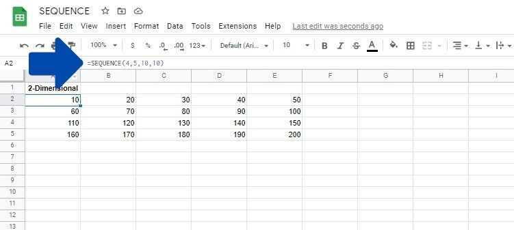
In this example, we will be using all four arguments to demonstrate the formula fully. Let’s pretend we want a sequence that will start from 10 and go up to 200 with a difference of 10 between every number. We also want to show our data on 4 rows and 5 columns. Here are the steps you need to follow to do this:
- Click on the cell where you wish to enter the formula. Ensure there are enough cells to contain the values for both the rows and columns.
- Enter =SEQUENCE(
- Now input the first and the second arguments, divided by a comma. The first argument is 4, while the second is 5 in this case—4 rows and 5 columns.
- In addition, we also will be using the start and the step argument. These both use the value of 10 as we want to start at 10 and increase by increments of 10 too.
- Finally, add the closing bracket and press Enter.
Date Array
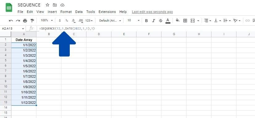
There are several clever ways to utilize this function, like nesting another function in the SEQUENCE formula. One method to do this is to create a sequence of dates. You can do this by using the DATE formula inside the SEQUENCE formula. Here are the steps you need to follow to do this:
- Write =SEQUENCE( in an empty cell, to start the formula.
- Write the row and column arguments divided by a comma. In our example, we are using 12 for the row argument and 1 for column.
- Now we need to write the start argument here. Instead, we start writing the date formula. In this case, we write DATE(2022,1,1).
- Add another comma and input the step argument. In this case, it is 1 to have single sequential days. If you wanted to do weeks, you could type 7 instead.
- Finally, add the closing bracket and press Enter.
You won't instantly see the date format, which you're used to. Instead, you will see a sequence of seemingly random numbers. To change the numbers into dates:
- Select the cells containing the numbers and click on Format.
- In the dropdown menu, click on Number and then Date.
You can also check out our guide to Google Sheets formatting to learn more.
Wrapping Up SEQUENCE in Google Sheets
SEQUENCE is a handy Google Sheets function that saves you time when building large spreadsheets. Although we used small-scale examples to make it simple to follow along, it’s easy to imagine how much easier this function makes life for those who have to make sizable sequential data sets frequently.
Yet, SEQUENCE is just the start of making the Google Suite easier to use. There are plenty of other tricks to save you time and effort.

