Number formatting is a core part of Excel for anyone who uses it often. Through these built-in formats, you can automatically add symbols to your cells, have different formats for positive or negative values, and much more.

Although the built-in Excel formats are useful, in some cases, they might not include the particular format that you're after. In that case, you can use custom formatting in Excel to create exactly the format you want for your cells.

Using Custom Formatting in Excel

The built-in number formats in Excel are many and useful, but what if the specific format that you want isn't included in the built-in formats?

For that, you'll have to create your own custom format in Excel. As a general note, you can customize nearly everything in Excel. You can even create a button with a custom function in Excel.

Creating custom number formats in Excel is not easy right-off the bat, but once you get the hang of the symbols and what they do, it'll be a breeze. To get started, check out the table below. This table is a summary of some important symbols in custom formatting.

Another important factor to consider when creating a custom format is the order. You can include different formats for positive numbers, negative numbers, and zero in your custom format by putting a semicolon (;) between them. Consider the format below:

        "Positive"; "Negative"; "Zero"
    

With this formatting applied, if the cell value is positive, the cell will display the string Positive. For negative values it will display Negative, and for zero it will display Zero. The custom format doesn't have to include all three of these conditions. If you put in only the first one, it will be used for all three.

What we talked about here isn't all that there is to custom formatting in Excel, but it's a good starting point. Now let's turn this knowledge into skill with some examples.

1. Excel Custom Formatting Example: Text Suffixes

To give you an understanding of custom formats in Excel, we're going to start with a simple example. Let's say that you want to input the duration of some operations into a range of cells.

By creating a custom format that adds an Hours suffix to the cell, you can simply just type in the numeral value of the years and skip having to type the text. Here's how you can do that:

1. In the Home tab, go to the Number section and click on General.
2. From the menu, select More Number Formats. This will open a new window.
3. In the new window, under Category, select Custom.
4. Select any of the formats.
5. Enter the line below under Type:

           # "Hours"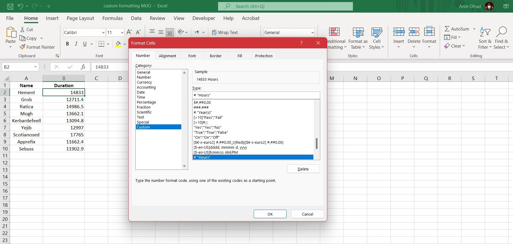
       

   

6. Press OK.

   

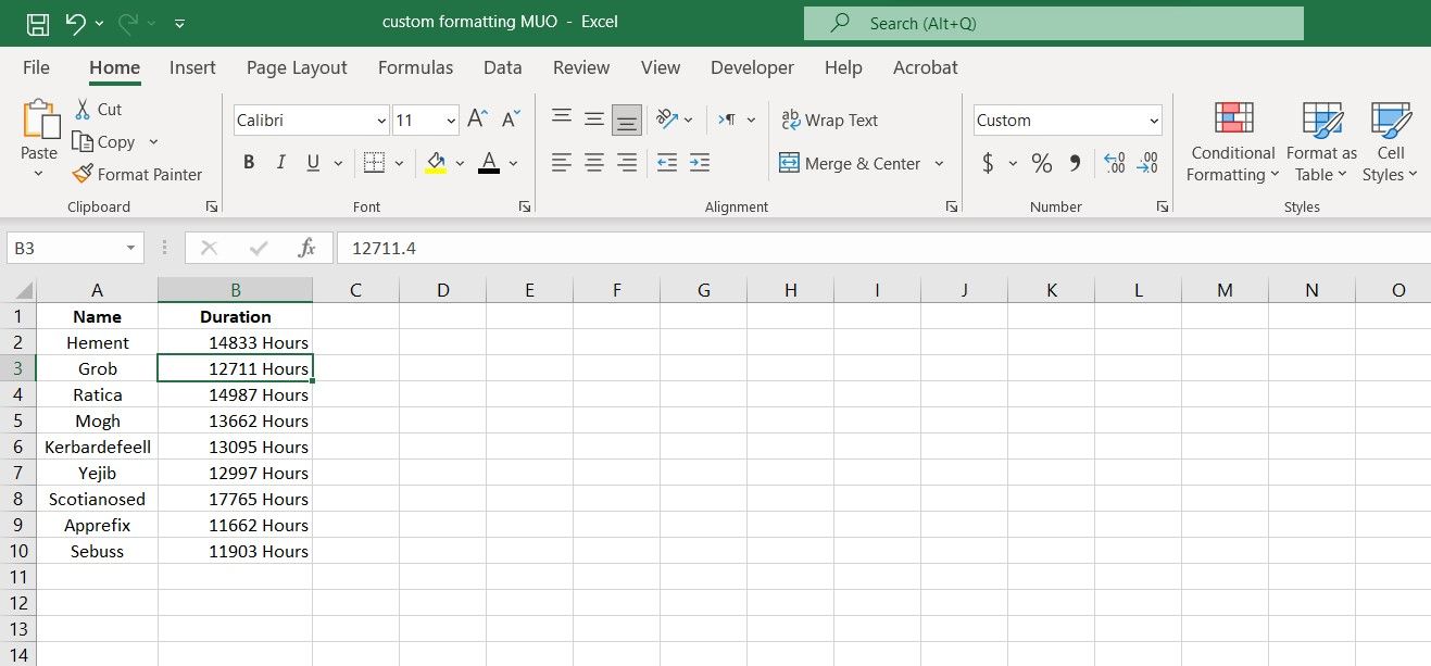
Now your custom format is ready. Select the cells that you want to apply this custom formatting on, then repeat the steps above and select the custom format that you just created. Notice how the cell values are unchanged despite the Hours suffix being displayed in the cells.

The hashtag (#) in the code represents any optional number, but since we didn't include any decimals in the format, the decimals aren't displayed in the cells. In fact, the numbers are all rounded up.

2. Excel Custom Formatting Example: Decimals and Thousands Separator

It's time we got an example of custom formatting for different values in Excel. As mentioned before, you can create different formats for positive, negative, and zero values in a single custom cell format.

Let's build on the previous example. Here we have the same spreadsheet, but want to change the displayed values for negatives and zeros. To improve the accuracy and the readability of the displayed numbers, we're also going to add a thousands separator and a decimal point.

1. In the Home tab, go to the Number section and click on General.
2. From the menu, select More Number Formats. This will open a new window.
3. In the new window, under Category, select Custom.
4. Select the format you created in the previous section.
5. Enter the line below under Type:

           ###,###.0 "Hours"; "Value is negative!"; "-"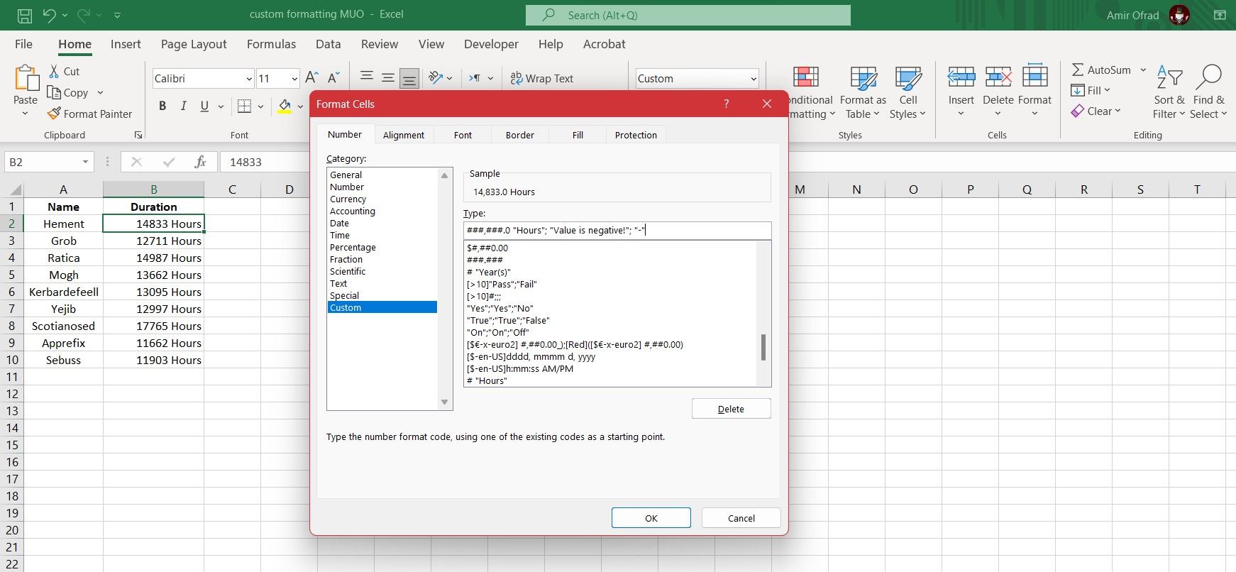
       

   

6. Click OK.

   

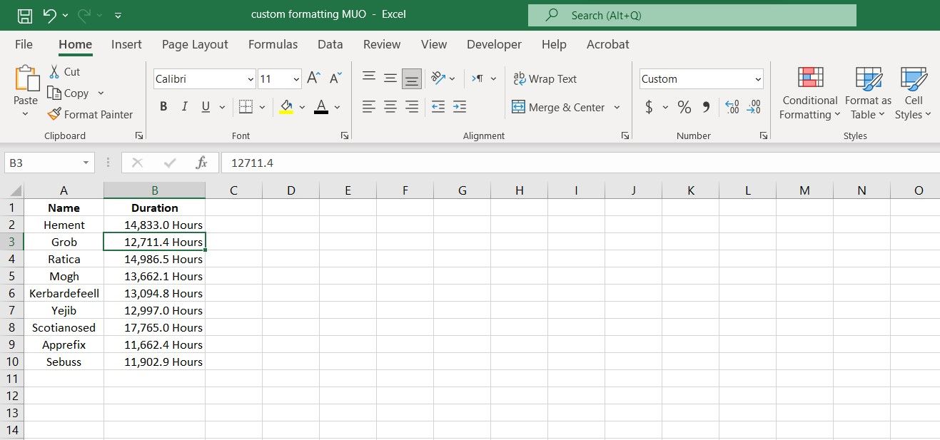
Now if you apply this format to the cells, you'll see that it adds the Hours suffix to the positive values, displays Value is negative! where the values are negative, and displays—for zeroes. Adding a decimal point to this custom format inhibited Excel from rounding the numbers, and the thousands separator has made the numbers easier to read.

Custom formats with text strings allow you to create new things in Excel. For instance, you can use custom formatting to create a bulleted list in Excel.

3. Excel Custom Formatting Example: Colors and Conditions

Now, let's try something new with custom formatting. In this example, we have the grades of some students. The grades are out of 20, and if a student has got 10 or above, they have passed the exam. If not, then they have unfortunately failed.

The goal here is to create a custom format that will display Pass in green if the cell value is 10 or above, and display Fail in red if the cell value is below 10.

As mentioned before, you can create custom conditions inside brackets ([ ]) and use brackets to specify font color. Let's get down to it. With that in mind, let's create a custom format with conditions.

1. In the new window, under Category, select Custom.
2. Select any of the formats.
3. Enter the line below under Type:

           [>=10][Green]"Pass";[<10][Red]"Fail"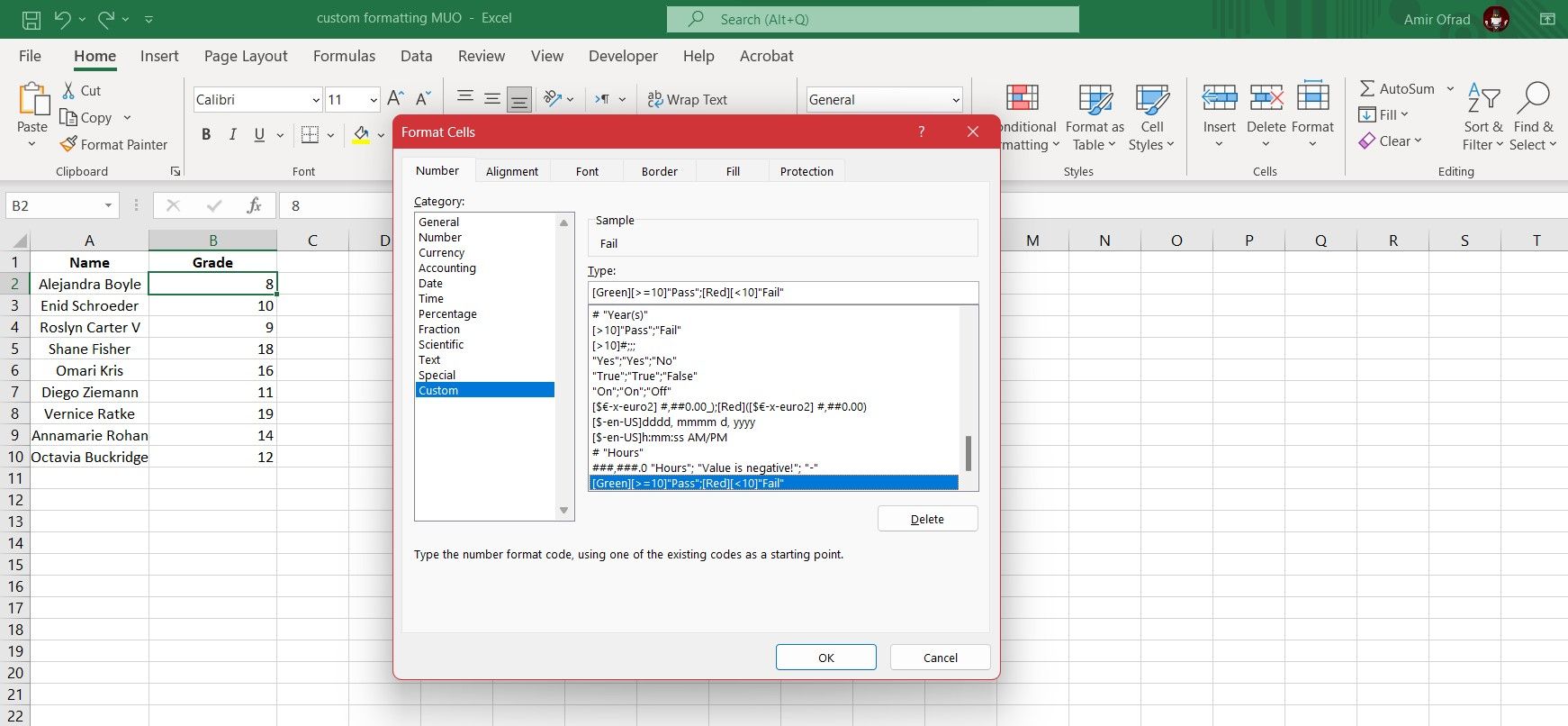
       

   

4. Click OK.

   

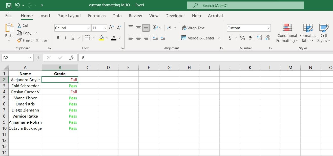
Once you apply the format to the cells, the cells below 10 will display Fail in red, and the rest will display Pass in green. Again, note that the cell values haven't changed from the original numbers.

Using custom formatting, you can keep the cell values intact and display text based on the cell values. If you're interested in using conditions for your custom formats, you should definitely check out conditional formatting in Excel.

Get What You Want From Excel

Excel is a tool designed to take the burden off your shoulders when it comes to dealing with data and numbers. Cell formatting is one Excel feature that provides help in this aspect, but if the formatting you want isn't listed in the Excel built-in formats, you don't have to compromise.

With custom formatting in Excel, you can create a unique cell format that exactly suits your needs. Now that you know enough to get started with custom cell formatting in Excel, it's time to experiment and improve your spreadsheets.