Microsoft Excel is a mainstay application for anyone who has to work with a lot of numbers, from students to accountants. But its usefulness extends beyond large databases; it can do a lot of great things with text, too. The functions listed below will help you analyze, edit, convert, and otherwise make changes to text—and save you many hours of boring and repetitive work.
Navigation: Non-Destructive Editing | Half- and Full-Width Characters | Character Functions | Text Analyzing Functions | Text Converting Functions | Text Editing Functions | Text Replacing Functions | Text Piecing Functions | A Real World Example
Non-Destructive Editing
One of the principles of using Excel text functions is that of non-destructive editing. Put simply, this means that whenever you use a function to make a change to the text in a row or column, that text will remain unchanged and the new text will be placed in a new row or column. This can be a bit disorienting at first, but it can be very valuable, especially if you're working with a huge spreadsheet that would be difficult or impossible to reconstruct if an edit goes wrong.
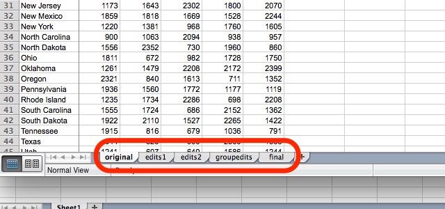
While you can continue adding columns and rows to your ever-expanding giant spreadsheet, one way to take advantage of this is to save your original spreadsheet in the first sheet in a document, and subsequent edited copies in other sheets. That way, no matter how many edits you make, you'll always have the original data that you're working from.
Half- and Full-Width Characters
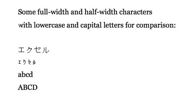
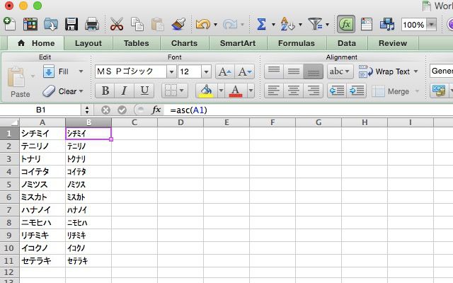
Some of the functions that are discussed here reference single- and double-byte character sets, and before we get started, it will be useful to clear up exactly what those are. In some languages, like Chinese, Japanese, and Korean, each character (or a number of characters) will have two possibilities for being displayed: one that's encoded in two bytes (known as a full-width character), and one that's encoded in a single byte (half-width). You can see the difference in these characters here:
As you can see, the double-byte characters are larger and, often, easier to read. However, in some computing situations, one or the other of these types of encodings is required. If you don't know what any of this means or why you'd need to worry about it, it's very likely that it's something you won't have to think about. In case you do, however, there are functions included in the following sections that relate specifically to half-width and full-width characters.
Character Functions
It's not very often that you work with single characters in Excel, but those situations do occasionally come up. And when they do, these functions are the ones you need to know.
The CHAR and UNICHAR Functions
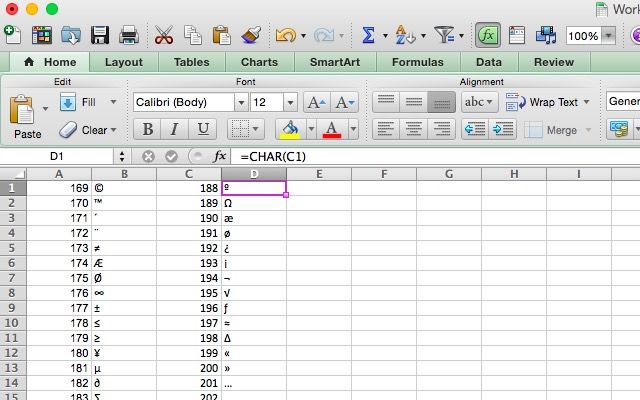
CHAR takes a character number and returns the corresponding character; if you have a list of character numbers, for example, CHAR will help you turn them into the characters that you're more used to dealing with. The syntax is quite simple:
=CHAR([text])
[text] can take the form of a cell reference or a character; so =CHAR(B7) and =CHAR(84) both work. Note that when using CHAR, it will use the encoding that your computer is set to; so your =CHAR(84) might be different than mine (especially if you're on a Windows computer, as I'm using Excel for Mac).
If the number that you're converting to is a Unicode character number, and you're using Excel 2013, you'll need to use the UNICHAR function. Previous versions of Excel don't have this function.
The CODE and UNICODE Functions
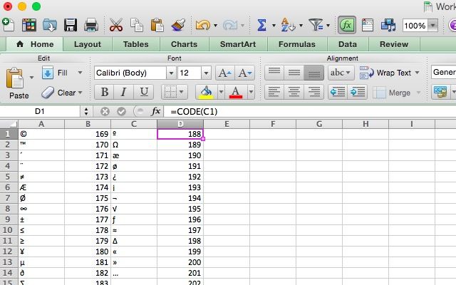
As you might expect, CODE and UNICODE do the exact opposite of the CHAR and UNICHAR functions: they take a character and return the number for the encoding that you've chosen (or that's set to the default on your computer). An important thing to keep in mind is that if you run this function on a string that contains more than one character, it will only return the character reference for the first character in the string. The syntax is very similar:
=CODE([text])
In this case, [text] is a character or a string. And if you want the Unicode reference instead of your computer's default, you'll use UNICODE (again, if you have Excel 2013 or later).
Text Analyzing Functions
The functions in this section will help you get information about the text in a cell, which can be useful in many situations. We'll start with the basics.
The LEN Function
LEN is a very simple function: it returns the length of a string. So if you need to count the number of letters in a bunch of different cells, this is the way to go. Here's the syntax:
=LEN([text])
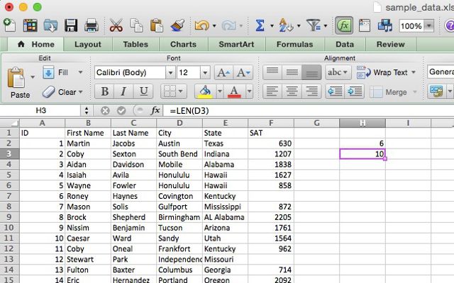
The [text] argument is the cell or cells that you'd like to count. Below, you can see that using the LEN function on a cell that contains the city name "Austin," it returns 6. When it's used on the city name "South Bend," it returns 10. A space counts as a character with LEN, so keep that in mind if you're using it to count the number of letters in a given cell.
The related function LENB does the same thing, but works with double-byte characters. If you were to count a series of four double-byte characters with LEN, the result would be 8. With LENB, it's 4 (if you have a DBCS enabled as the default language).
The FIND Function
You may wonder why you'd use a function called FIND if you can just use CTRL+F or Edit > Find. The answer lies in the specificity with which you can search using this function; instead of searching the entire document, you can choose at which character of each string the search begins. The syntax will help clear up this confusing definition:
=FIND([find_text], [within_text], [start_num])
[find_text] is the string that you're looking for. [within_text] is the cell or cells in which Excel will look for that text, and [start_num] is the first character that it will look at. It's important to note that this function is case-sensitive. Let's take an example.
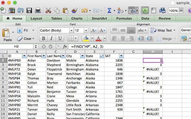
I've updated the sample data so that the ID number of each student is a six-character alphanumeric sequence, each of which begins with a single digit, an M for "male," a sequence of two letters to indicate the student's performance level (HP for high, SP for standard, LP for low, and UP/XP for unknown), and a final sequence of two numbers. Let's use FIND to highlight each high-performing student. Here's the syntax we'll use:
=FIND("HP", A2, 3)
This will tell us whether HP appears after the third character of the cell. Applied to all of the cells in the ID column, we can see at a glance whether the student was high-performing or not (note that the 3 returned by the function is the character at which HP is found). FIND can be put to better use if you have a wider variety of sequences, but you get the idea.
As with LEN and LENB, FINDB is used for the same purpose as FIND, only with double-byte character sets. This is important because of the specification of a certain character. If you're using a DBCS and you specify the fourth character with FIND, the search will begin at the second character. FINDB solves the problem.
Note that FIND is case-sensitive, so you can search for a specific capitalization. If you'd like to use a non-case-sensitive alternative, you can use the SEARCH function, which takes the same arguments and returns the same values.
The EXACT Function
If you need to compare two values to see if they're the same, EXACT is the function you need. When you supply EXACT with two strings, it will return TRUE if they're exactly the same, and FALSE if they're different. Because EXACT is case-sensitive, it will return FALSE if you give it strings that read "Test" and "test." Here's the syntax for EXACT:
=EXACT([text1], [text2])
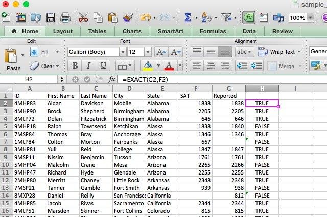
Both arguments are pretty self-explanatory; they're the strings that you'd like to compare. In our spreadsheet, we'll be using them to compare two SAT scores. I've added a second row and called it "Reported." Now we'll go through the spreadsheet with EXACT and see where the reported score differs from the official score using the following syntax:
=EXACT(G2,F2)
Repeating that formula for each row in the column gives us this:
Text Converting Functions
These functions take the values from one cell and turn them into another format; for example, from a number to a string or from a string to a number. There are a few different options for how you go about this and what the exact result is.
The TEXT Function
TEXT converts numerical data into text and allows you to format it in specific ways; this could be useful, for example, if you're planning on using Excel data in a Word document. Let's look at the syntax and then see how you might use it:
=TEXT([text], [format])
The [format] argument lets you choose how you'd like the number to appear in text. There are a number of different operators that you can use to format your text, but we'll stick to a simple ones here (for full details, see the Microsoft Office help page on TEXT). TEXT is often used to convert monetary values, so we'll start with that.
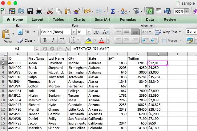
I've added a column called "Tuition" that contains a number for each student. We'll format that number into a string that looks a bit more like we're used to reading monetary values. Here's the syntax we'll use:
=TEXT(G2,"$#,###")
Using this formatting string will give us numbers that are preceded by the dollar symbol and include a comma after the hundreds place. Here's what happens when we apply it to the spreadsheet:
Each number is now correctly formatted. You can use TEXT to format numbers, currency values, dates, times, and even to get rid of insignificant digits. For details on how to do all of these things, check out the help page linked above.
The FIXED Function
Similar to TEXT, the FIXED function takes input and formats it as text; however, FIXED specializes in converting numbers into text and giving you a few specific options for formatting and rounding the output. Here's the syntax:
=FIXED([number], [decimals], [no_commas])
The [number] argument contains the reference to the cell that you'd like to convert to text. [decimals] is an optional argument that allows you to choose the number of decimals that are retained in the conversion. If this is 3, you'll get a number like 13.482. If you use a negative number for decimals, Excel will round the number. We'll take a look at that in the example below. [no_commas], if set to TRUE, will exclude commas from the final value.
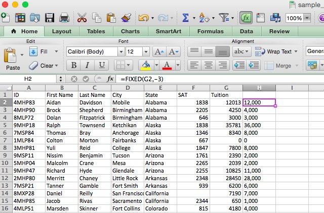
We'll use this to round the tuition values that we used in the last example to the nearest thousand.
=FIXED(G2, -3)
When applied to the row, we get a row of rounded tuition values:
The VALUE Function
This is the opposite of the TEXT function—it takes any cell and turns it into a number. This is especially useful if you import a spreadsheet or copy and paste a large amount of data and it gets formatted as text. Here's how to fix it:
=VALUE([text])
That's all there is to it. Excel will recognize accepted formats of constant numbers, times, and dates and will convert them to numbers that can then be used with numerical functions and formulas. This is a pretty simple one, so we'll skip the example.
The DOLLAR Function
Similar to the TEXT function, DOLLAR converts a value to text—but it also adds a dollar sign. You can choose the number of decimals to include, as well:
=DOLLAR([text], [decimals])
If you leave the [decimals] argument blank, it will default to 2. If you include a negative number for the [decimals] argument, the number will be rounded to the left of the decimal.
The ASC Function
Remember our discussion of single- and double-byte characters? This is how you convert between them. Specifically, this function converts full-width, double-byte characters into half-width, single-byte ones. It can be used to save some space in your spreadsheet. Here's the syntax:
=ASC([text])
Pretty simple. Just run the ASC function on any text that you'd like converted. To see it in action, I'll be converting this spreadsheet, which contains a number of Japanese katakana—these are often rendered as full-width characters. Let's change them to half-width.
The JIS Function
Of course, if you can convert one way, you can also convert back the other way. JIS converts from half-width characters to full-width ones. Just like ASC, the syntax is very simple:
=JIS([text])
The idea's pretty simple, so we'll move on to the next section without an example.
Text Editing Functions
One of the most useful things you can do with text in Excel is to programmatically make edits to it. The following functions will help you take text input and get into the exact format that's most useful to you.
The UPPER, LOWER, and PROPER Functions
These are all very simple functions to understand. UPPER makes text uppercase, LOWER makes it lowercase, and PROPER capitalizes the first letter in each word while leaving the rest of the letters lowercase. There's no need for an example here, so I'll just give you the syntax:
=UPPER/LOWER/PROPER([text])
Choose the cell or range of cells that your text is in for the [text] argument, and you're set to go.
The CLEAN Function
Importing data into Excel usually goes pretty well, but sometimes you end up with characters that you don't want. This is most common when there are special characters in the original document that Excel can't display. Instead of going through all of the cells that contain those characters, you can use the CLEAN function, which looks like this:
=CLEAN([text])
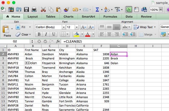
The [text] argument is simply the location of the text that you want to clean. In the example spreadsheet, I've added a few non-printable characters to the names in Column A that need to be gotten rid of (there's one in row 2 that pushes the name to the right, and an error character in row 3). I've used the CLEAN function to transfer the text to Column G without those characters:
Now, Column G contains the names without the non-printable characters. This command isn't just useful for text; it can often help you out if numbers are messing up your other formulas, too; special characters can really wreak havoc with calculations. It's essential when you're converting from Word to Excel, though.
The TRIM Function
While CLEAN gets rid of non-printable characters, TRIM gets rid of extra spaces at the beginning or end of a text string you might end up with these if you copy text over from a Word or a plain text document, and end up with something like " Follow-up Date " . . . to turn it into "Follow-up Date," just use this syntax:
=TRIM([text])
When you use it, you'll see similar results to when you use CLEAN.
Text Replacing Functions
Occasionally, you'll need to replace specific strings in your text with a string of other characters. Using Excel formulas is much faster than find and replace, especially if you're working with a very large spreadsheet.
The SUBSTITUTE Function
If you're working with a lot of text, sometimes you'll need to make some major changes, like subbing out one string of text for another. Maybe you realized that the month is wrong in a string of invoices. Or that you typed someone's name incorrectly. Whatever the case, sometimes you need to replace a string. That's what SUBSTITUTE is for. Here's the syntax:
=SUBSTITUTE([text], [old_text], [new_text], [instance])
The [text] argument contains the location of the cells you want to do the replacing in, and the [old_text] and [new_text] are pretty self-explanatory. [instance] allows you to specify a specific instance of the old text to replace. So if you want to replace only the third instance of the old text, you'd enter "3" for this argument. SUBSTITUTE will copy over all other values (see below).
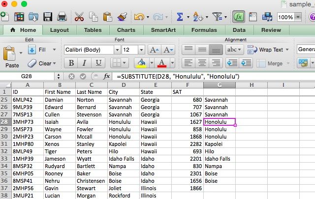
As an example, we'll correct a spelling error in our spreadsheet. Let's say "Honolulu" was accidentally spelled as "Honululu." Here's the syntax we'll use to correct it:
=SUBSTITUTE(D28, "Honululu", "Honolulu")
And here's what happens when we run this function:
After dragging the formula into the surrounding cells, you'll see that all of the cells from column D were copied over, except those that contained the misspelling "Honululu," which were replaced with the correct spelling.
The REPLACE Function
REPLACE is a lot like SUBSTITUTE, but instead of replacing a specific string of characters, it will replace the characters in a specific position. A look at the syntax will make it clear how the function works:
=REPLACE([old_text], [start_num], [num_chars], [new_text])
[old_text] is where you'll specify the cells that you want to replace text in. [start_num] is the first character that you'd like to replace, and [num_chars] is the number of characters that will be replaced. We'll see how this works in just a moment. [new_text], of course, is the new text that will be inserted into the cells—this can also be a cell reference, which can be quite useful.
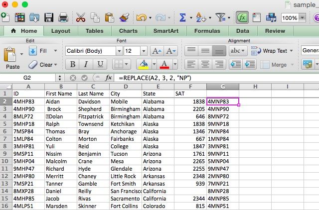
Let's take a look at an example. In our spreadsheet, the student IDs have HP, SP, LP, UP, and XP sequences. We want to get rid of them and change them all to NP, which would take a long time using SUBSTITUTE or Find and Replace. Here's the syntax we'll use:
=REPLACE(A2, 3, 2, "NP")
Applied to the whole column, here's what we get:
All of the two-letter sequences from Column A have been replaced with "NP" in column G.
Text Piecing Functions
In addition to making changes to strings, you can also do things with smaller pieces of those strings (or use those strings as smaller pieces to make up larger ones). These are some of the most commonly used text functions in Excel.
The CONCATENATE Function
This is one that I've used quite a few times myself. When you have two cells that need to be added together, CONCATENATE is your function. Here's the syntax:
=CONCATENATE([text1], [text2], [text3]...)
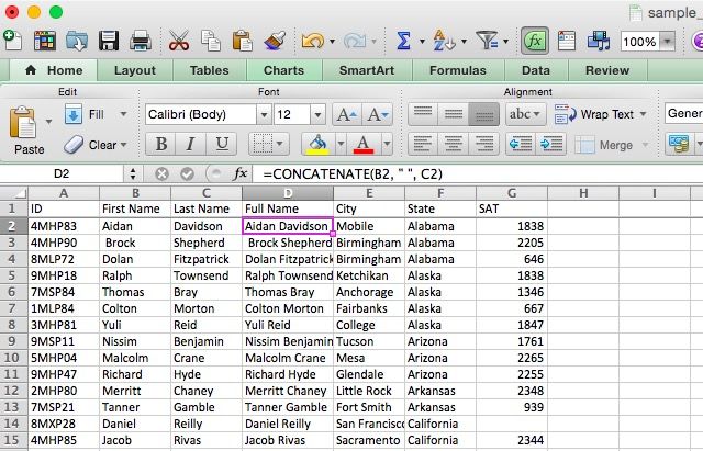
What makes concatenate so useful is that the [text] arguments can be plain text, like "Arizona," or cell references like "A31." You can even mix the two. This can save you a huge amount of time when you need to combine two columns of text, like if you need to create a "Full Name" column from a "First Name" and a "Last Name" column. Here's the syntax we'll use to do that:
=CONCATENATE(A2, " ", B2)
Notice here that the second argument is a blank space (typed as quotation-mark-space-qoutation-mark). Without this, the names would be concatenated directly, with no space between first and last names. Let's see what happens when we run this command and use autofill on the rest of the column:
Now we have a column with everyone's full name. You can easily use this command to combine area codes and phone numbers, names and employee numbers, cities and states, or even currency signs and amounts.
You can shorten the CONCATENATE function to a single ampersand in most cases. To create the formula above using the ampersand, we'd type this:
=A2 & " " & B2
You can also use it to combine cell references and lines of text, like this:
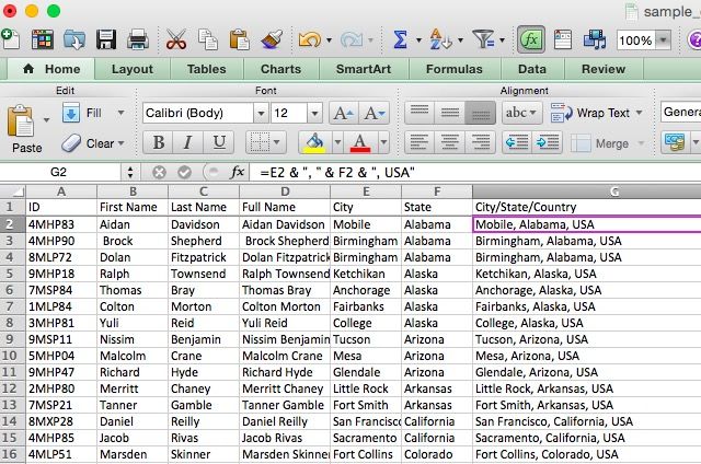
=E2 & ", " & F2 & ", USA"
This takes the cells with city and state names and combines them with "USA" to get full address, as seen below.
The LEFT and RIGHT Functions
Often, you want to work with just the first (or last) few characters of a text string. LEFT and RIGHT let you do that by returning only a certain number of characters starting from the left- or rightmost character in a string. Here's the syntax:
=LEFT/RIGHT([text], [num_chars])
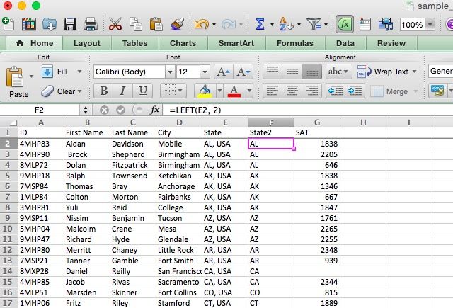
[text], of course, is the original text, and [num_chars] is the number of characters you'd like to return. Let's take a look at an example of when you might want to do this. Let's say that you've imported a number of addresses, and each contains both the state abbreviation and the country. We can use LEFT to get just the abbreviations, using this syntax:
=LEFT(E2, 2)
Here's what that looks like applied to our spreadsheet:
If the abbreviation had come after the state, we would have used RIGHT in the same way.
The MID Function
MID is a lot like LEFT and RIGHT, but lets you pull characters out of the middle of a string, starting at a position you specify. Let's take a look at the syntax to see exactly how it works:
=MID([text], [start_num], [num_chars])
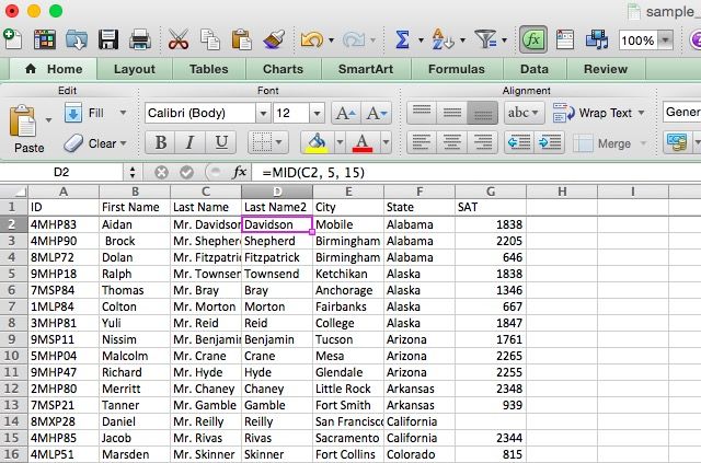
[start_num] is the first character that will be returned. This means that if you want the first character in a string to be included in the result of a function, this will be "1." [num_chars] is the number of characters after the starting character that will be returned. We'll do a bit of text cleaning with this. In the example spreadsheet, we now have titles added to the last names, but we'd like to strip those out so that a last name of "Mr. Martin" will be returned as "Martin." Here's the syntax:
=MID(A2, 5, 15)
We'll use "5" as the start character, because the first letter of the person's name is the fifth character ("Mr. " takes up four spaces). The function will return the next 15 letters, which should be enough to not cut off the last part of anyone's name. Here's the result in Excel:
In my experience, I find MID to be most useful when you combine it with other functions. Let's say that this spreadsheet, instead of only including men, also included women, who could have either "Ms." or "Mrs." for their titles. What would we do then? You can combine MID with IF to get the first name regardless of title:
=IF(LEFT(A2, 3)="Mrs", MID(A2, 6, 16), MID(A2, 5, 15)
I'll let you figure out exactly how this formula works its magic (you may need to review Excel's boolean operators).
The REPT Function
If you need to take a string and repeat it a number of times, and you'd rather not type it over and over, REPT can help. Give REPT a string ("abc") and a number (3) of times that you want it repeated, and Excel will give you exactly what you asked for ("abcabcabc"). Here's the very easy syntax:
=REPT([text], [number])
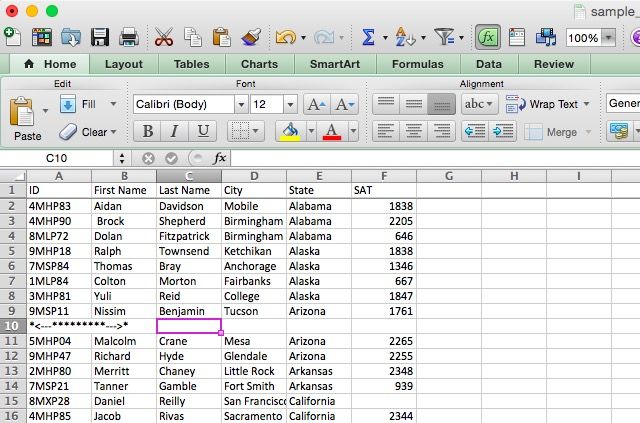
[text], obviously, is the base string; [number] is the number of times you want it repeated. While I haven't run into a good use of this function yet, I'm sure someone out there could use it for something. We'll use an example that, while it isn't exactly useful, could show you the potential of this function. We're going to combine REPT with "&" to create something new. Here's the syntax:
="*<---" & REPT("*", 9) & "--->*"
The result is shown below:
A Real-World Example
To give you an idea of how you might put a text function into use in the real world, I'll provide an example of where I combined MID with several conditionals in my own work. For my post-grad psychology degree, I ran a study in which participants had to click on one of two buttons, and the coordinates of that click were recorded. The button on the left of the screen was labelled A, and the one on the right was labelled B. Each trial had a correct answer, and each participant did 100 trials.
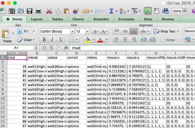
To analyze this data, I needed to see how many trials each participant got right. Here's what the results spreadsheet looked like, after a bit of cleaning:
The correct answer for each trial is listed in column D, and the coordinates of the click are listed in columns F and G (they're formatted as text, which complicated matters). When I started, I simply went through and did the analysis manually; if column D said "optiona" and the value in column F was negative, I would enter 0 (for "wrong"). If it was positive, I'd enter 1. The opposite was true if column D read "optionb."
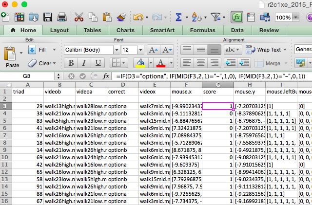
After a bit of tinkering, I came up with a way to use the MID function to do the job for me. Here's what I used:
=IF(D3="optiona", IF(MID(F3,2,1)="-",1,0), IF(MID(F3,2,1)="-",0,1))
Let's break that down. Starting with the first IF statement, we have the following: "if cell D3 says 'optiona', then [first conditional]; if not, then [second conditional]." The first conditional says this: "if the second character of cell F3 is a hyphen, return true; if not, return false." The third says "if the second character of cell F3 is a hyphen, return false; if not, return true."
It might take a while to wrap your head around this, but it should become clear. In short, this formula checks to see if D3 says "optiona"; if it does, and the second character of F3 is a hyphen, the function returns "true." If D3 contains "optiona" and the second character of F3 isn't a hyphen, it returns "false." If D3 doesn't contain "optiona" and the second character of F3 is a hyphen, it returns "false." If D3 doesn't say "optiona" and the second character of F2 isn't a hyphen, it returns "true."
Here's what the spreadsheet looks like when you run the formula:
Now, the "score" column contains a 1 for every trial the participant answered correctly and a 0 for every trial they answered incorrectly. From there, it's easy to sum up the values to see how many they got right.
I hope this example gives you an idea of how you can creatively use text functions when you're working with different types of data. Excel's power is nearly limitless, and if you take the time to come up with a formula that will do your job for you, you can save a ton of time and effort!
Excel Text Mastery
Excel is a powerhouse when it comes to working with numbers, but it has a surprising number of useful text functions as well. As we've seen, you can analyze, convert, replace, and edit text, as well as combine these functions with others do some complex calculations and transformations.
From sending email to doing your taxes, Excel can help you manage your entire life. And learning to use these text functions will bring you one step closer to being an Excel master.
Let us know how you have used text operations in Excel! What's the most complex transformation you have done?


