Microsoft Excel is a vibrant tool that is used for both business and personal tasks. One robust feature is called conditional formatting. This can come in handy for everyday situations as well as work-related ones.
We'll be taking a look at some general uses for conditional formatting, how to set them up, and of course, exploring a variety of tasks this feature is capable of doing.
Conditional Formatting Explained
Conditional formatting is a tool that can be used to apply a certain format to cells based on the data entered. For instance, you can color-code or highlight cells based on a set of rules.
Format Cells Using a Single Rule
You can apply this feature when you want to format cells based on one specific condition. If you want the cell to be highlighted in red every time you enter the letter A, this is a simple setup.
Format Cells Using Multiple Rules
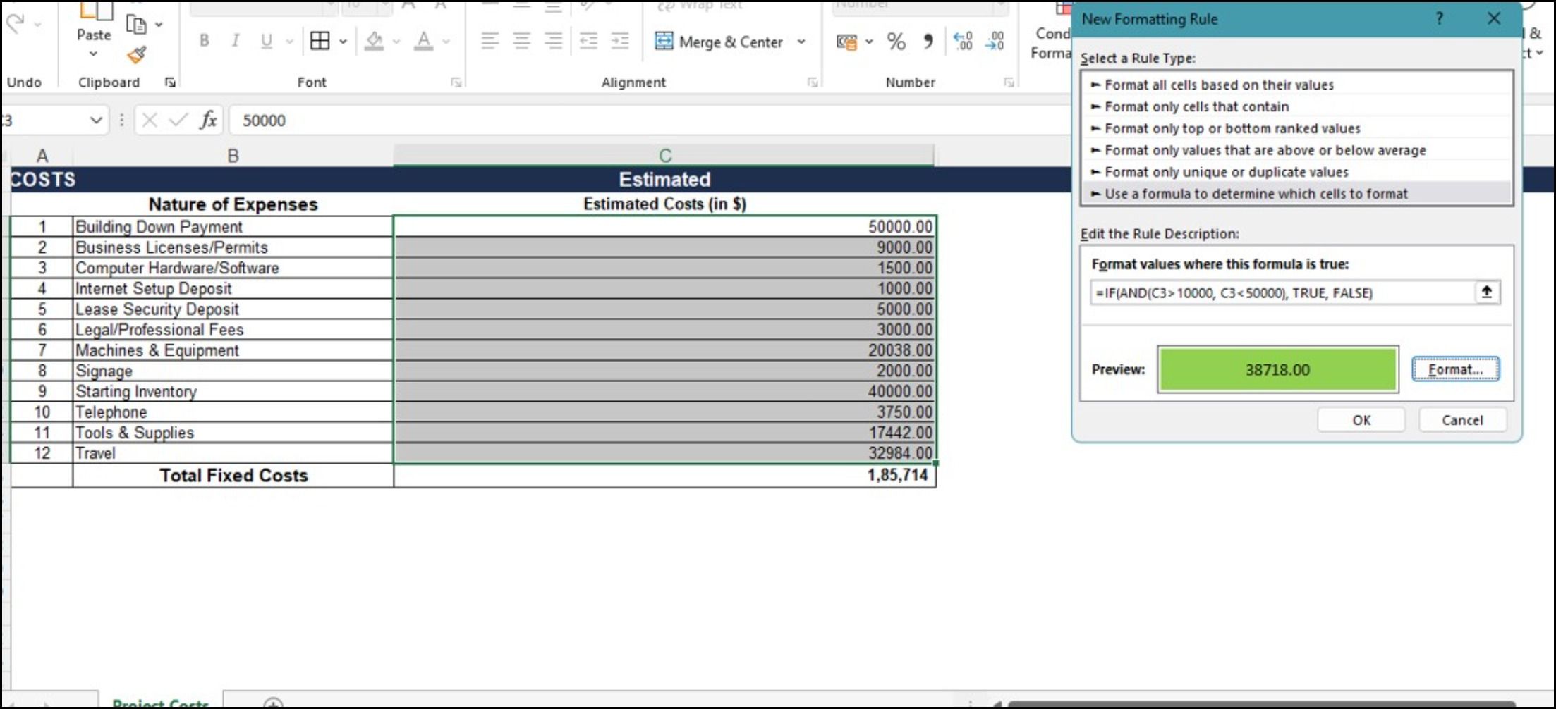
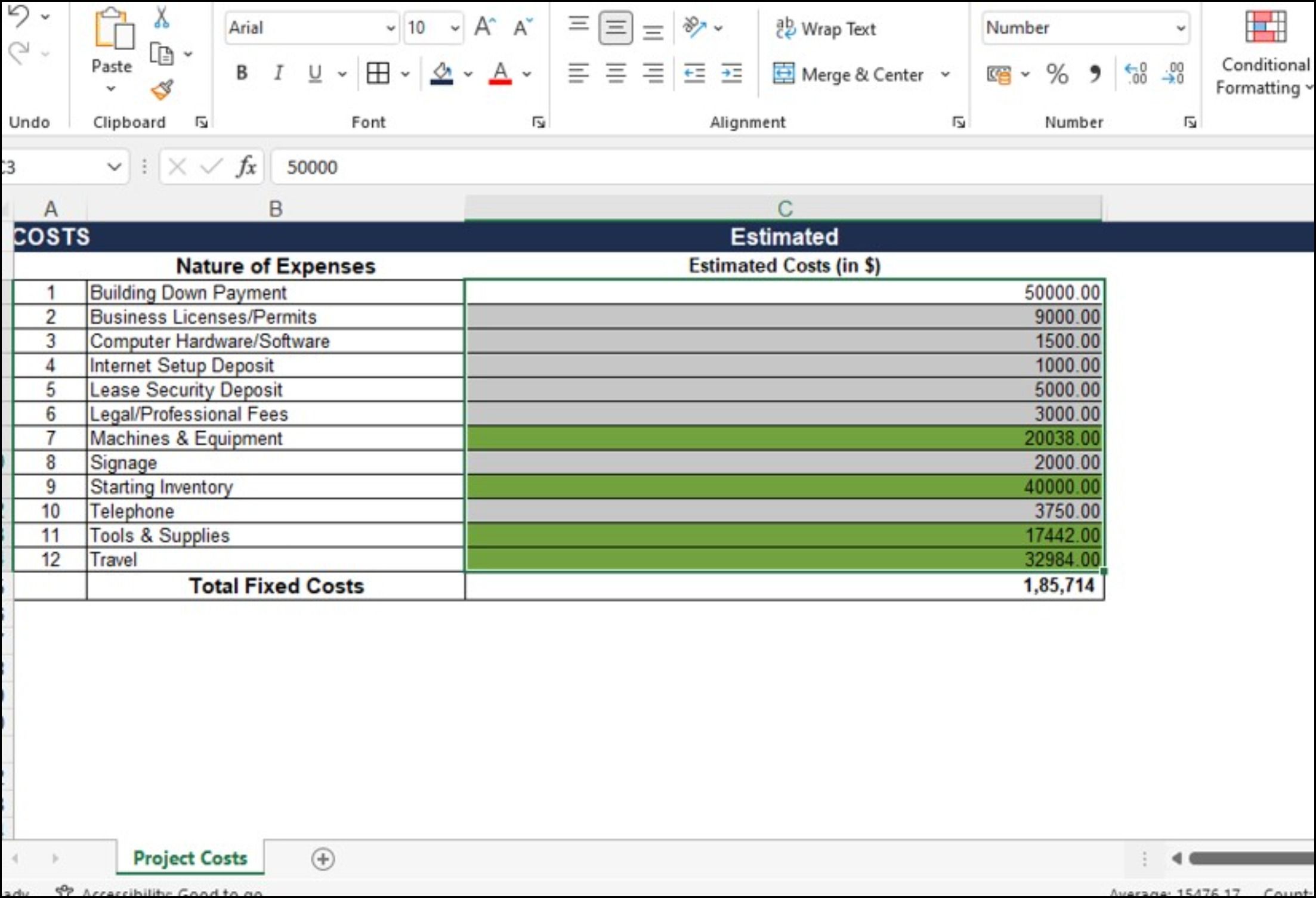
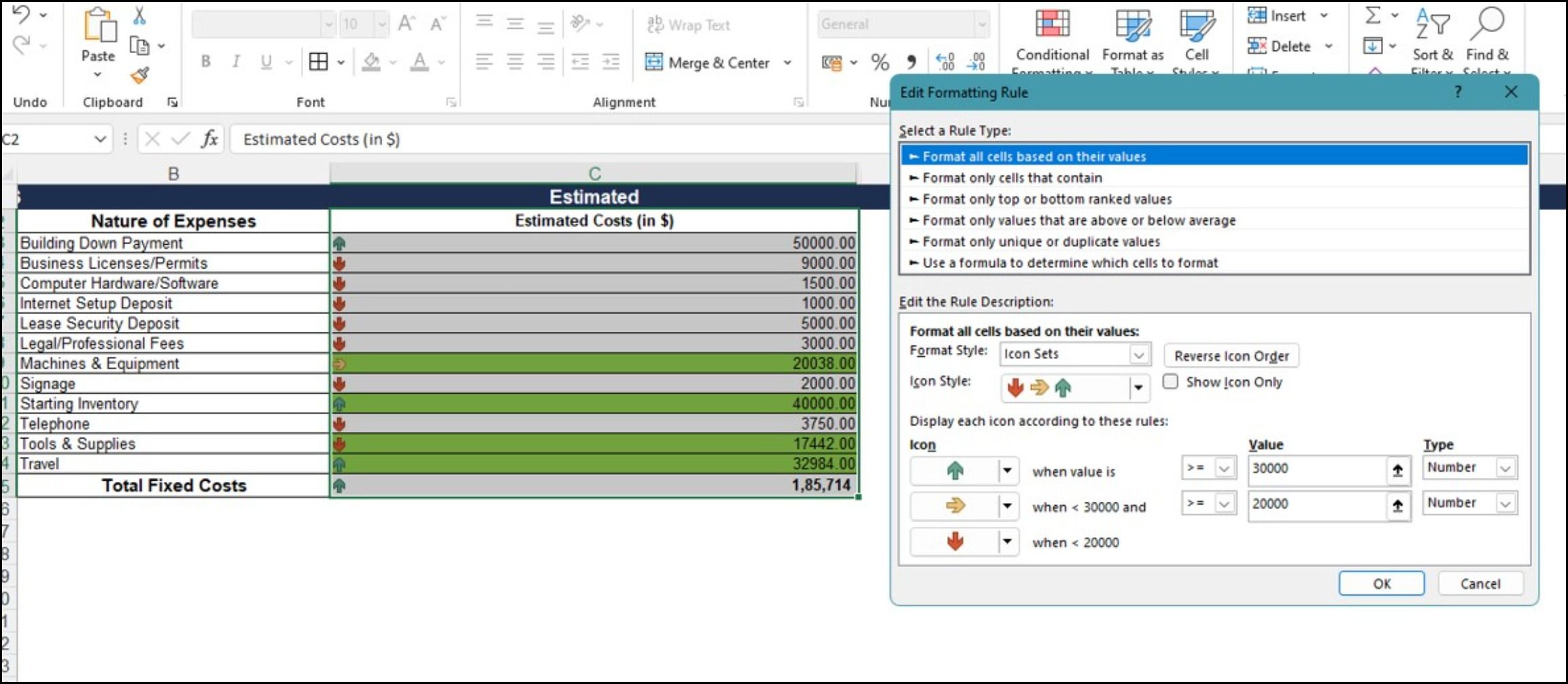
You might want to apply multiple rules to cells based on a set of conditions. Let's say you wish to cut down project expenses, so you can try to apply formatting in the Estimated Costs column to automatically highlight values between $10000 and $50000.
Here, you can use a nested formula—IF and AND functions to format cells. It's easy to do this:
- Select the cells to apply conditional formatting rules.
- Click on the Home tab > Conditional Formatting > New Rule.
-
From the dropdown options, select Use a formula to determine which cells to format, and enter the following formula:
=IF(AND(C3>10000, C3<50000), TRUE, FALSE)
- Head over to Format > Fill and choose a fill color to use, and click OK.
The tool has a variety of settings, options, and rules that can save time in spotting important items. It can also be advantageous for everyday tasks for school, home, work, and personal activities.
For School: Keep Things Simpler
You can keep track of your assignments, due dates, and grades in Excel. It's easy to apply formatting to highlight what is overdue, due tomorrow, or due in the next month, and it just takes a couple of steps:
- Select the cells where you will be adding the due dates.
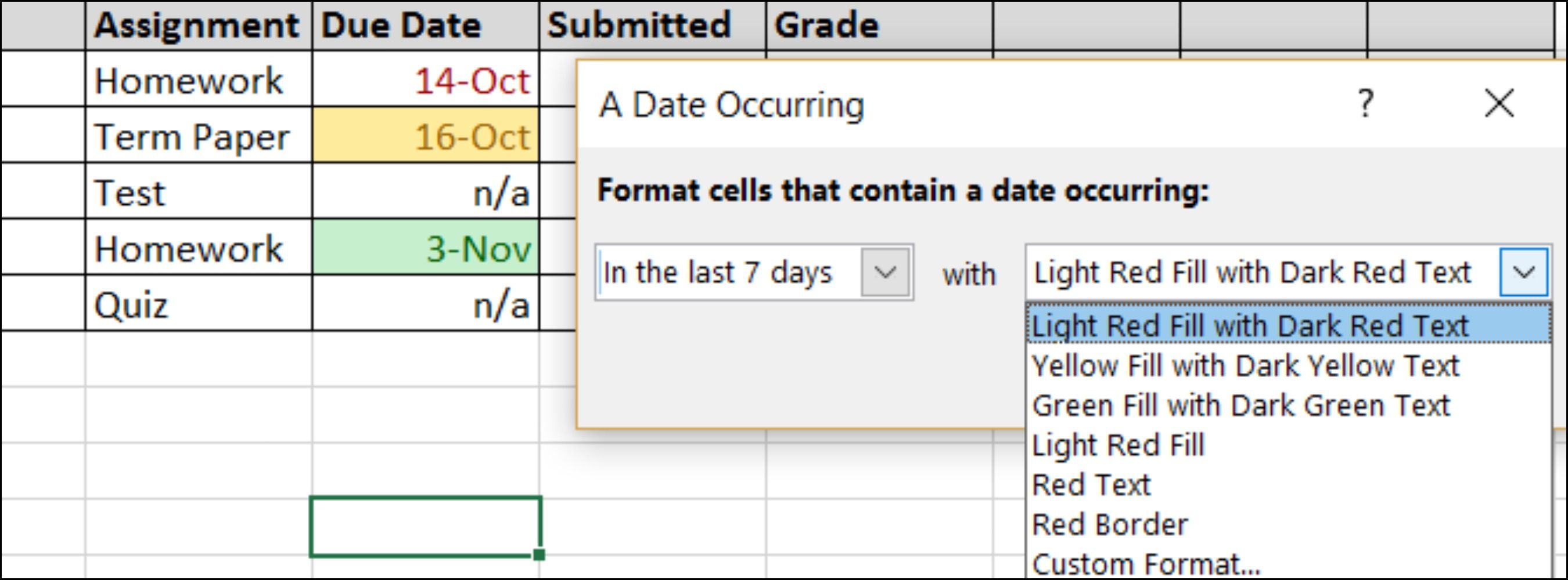
- Go to the Home tab > Conditional Formatting > Highlight Cells Rules > A Date Occurring.
- Then, choose your criteria, such as In the last 7 days with Red Text and Tomorrow with Yellow Fill.
This will help you see those important dates quickly. Assignments that are overdue or due shortly will pop right out.
For grade tracking, you can apply formatting for both letter and number grades that include a range.
- Select the cells where you will be adding the grades.
- Navigate to Home > Conditional Formatting > Highlight Cells Rules > Between.
- Then, add your values such as between C and F or 0 and 2 with Red Fill.
This gives you a nice and simple way to see how well your classes are going and where your grades are lower.
For Home: Highlight What's Important
Excel's conditional formatting feature can be just as helpful for managing finances, home projects, and task lists. If you feel like you're running behind on everything all the time, why not organize your life with these spreadsheet templates?
Manage Your Finances
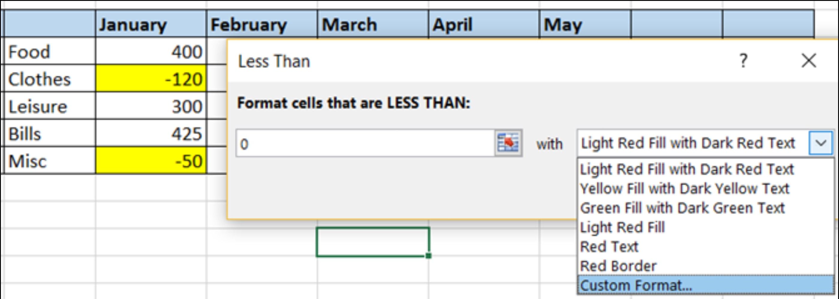
If you use it for your monthly budget, you can spot trouble quickly. Whether you have created your own spreadsheet or are using a handy template, applying formatting to negative numbers automatically is useful.
- Select the cells where you will be entering the numbers or formulas.
- Click Conditional Formatting on the Home tab > Conditional Formatting > Highlight Cells Rules > Less Than.
- Then, add 0 with the highlight you would like. In this example, we selected Custom Format with Yellow Fill to make those cells noticeable.
You can apply any type of formatting to make it more noticeable to you, from highlight to text to border color.
Create Personal To-Do Lists
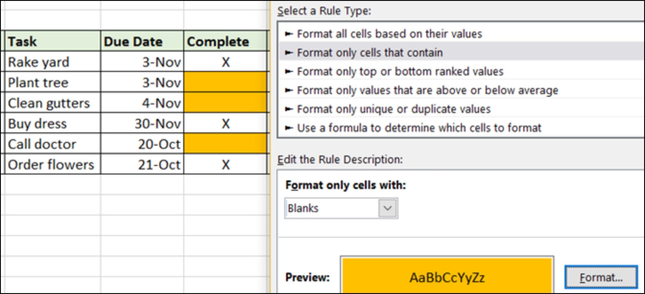
There is no better way to see completed and pending items on your to-do lists than with automatic formatting. With this approach, any task that is not marked completed with an X will be highlighted.
- Select the cells where you will be entering the completed indicator (X).
- Click on the Home tab > Conditional Formatting > Highlight Cells Rules > More Rules.
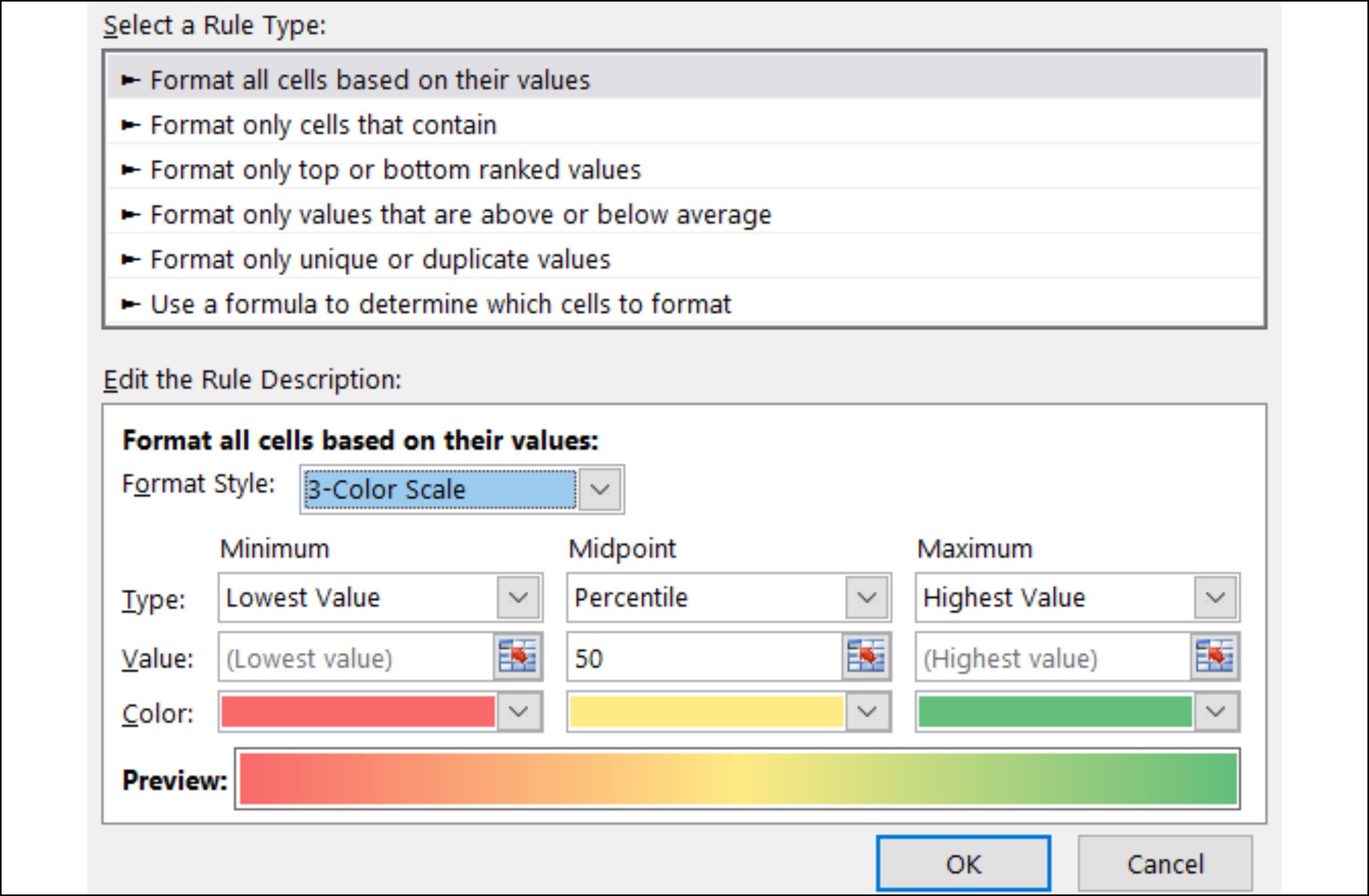
- In the pop-up window, choose Format only cells that contain.
- At the bottom, under Edit the Rule Description, select Blanks from the drop-down box.
- Then, select Format to pick the highlight color (orange, for instance) and click OK.
Applying this formatting takes only a minute and can be very helpful for keeping track of tasks that you have yet to complete.
For Personal Use: Make Goals Pop
Many people keep careful track of their personal goals with spreadsheet templates. From workout sessions to calorie counting, you can see how well you are meeting those goals with some cool formatting options.
Track Your Calories
For tracking calorie intake, apply formatting to see when you go over or under your goal for the day. In this instance, we will apply two separate rules.
- Select the cells where you will be entering the number of calories.
- Click the Home tab > Conditional formatting > Highlight Cells Rules > Greater Than.
- Then, add the calorie goal number with the highlight you would like. In this example, we selected 200 with Red Fill. This will show when we go above the calorie limit.
Next, set up the rule for going below the calorie limit.
- Select the same cells as in the first rule.
- Navigate to the Home tab > Conditional Formatting > Highlight Cells Rules > Less Than.
- Then, add the calorie goal number with the highlight you would like. In this example, we selected 200 with Green Fill.
Keep in mind that in this example, if you enter the exact number 200 for the calorie count, no formatting will be applied. This is because the number falls under neither rule.
For Business: Bring Out the Boldness
For those who work remotely or as independent contractors, Excel may be used for such tasks as time tracking or project estimates. Here's how you can do this:
Apply Time Tracking With Data Bars
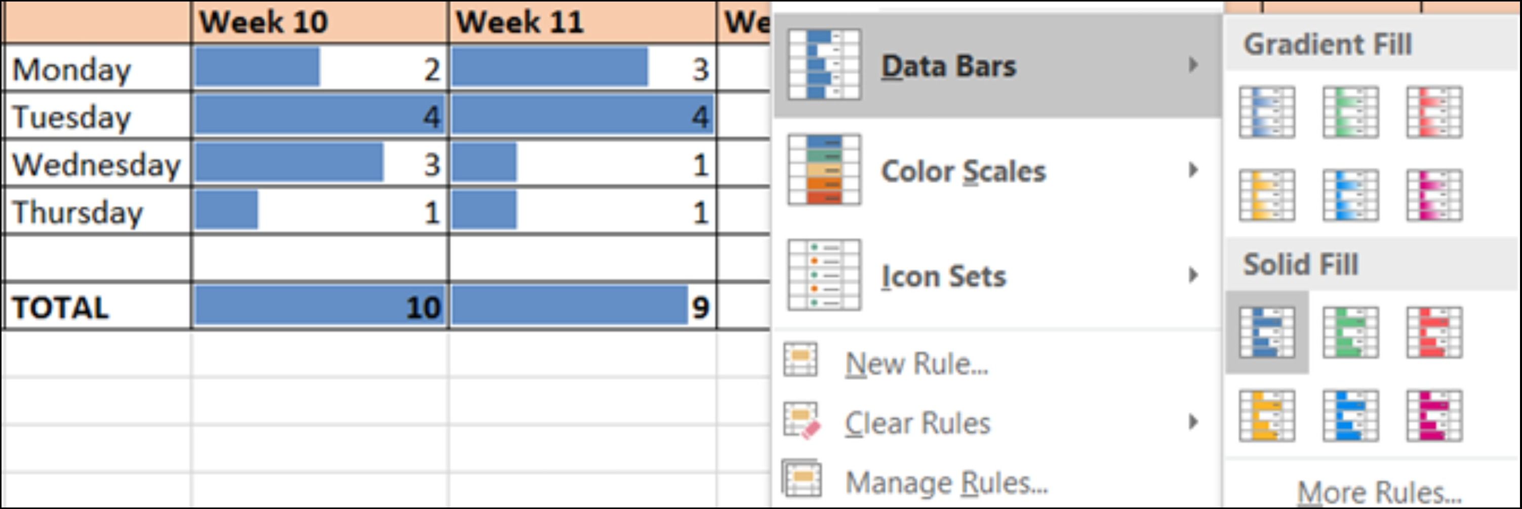
With a convenient way to keep track of hours worked as well as see a monthly or weekly overview, formatting with data bars can be quite useful.
- Select the cells where you will be entering the number of hours.
- Click Home tab > Conditional Formatting > Data Bars > Gradient Fill or Solid Fill, depending on your preference.
- Once you enter numbers into the designated cells, you will see the data bar adjust. The lower the number, the smaller the bar and vice versa. You can also apply the formatting to the totals you have calculated at the bottom.
This is a super-easy way to see your heaviest and lightest work days, weeks, or months.
Manage Project Priorities Using Icons and Shapes
Another great use of conditional formatting for business is for managing projects using Excel. Using indicator shapes and highlighting for items such as priority and effort can be beneficial when sharing the data with others.
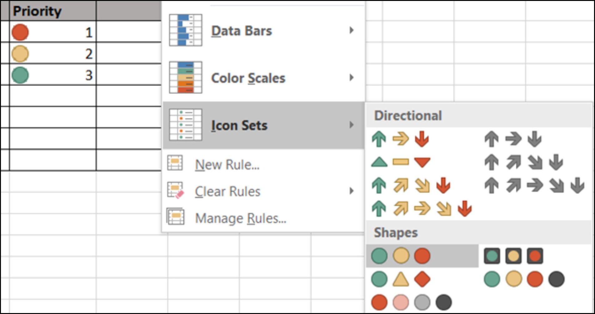
For setting priorities using numbers with 1 as the highest priority in red and 3 as the lowest in green, you can apply shape formatting.
- Select the cells where you'll be entering the numbers.
- Navigate to the Home tab > Conditional Formatting > Icon Set.
- Select the shapes you would like to use.
As you enter the numbers 1, 2, and 3, you will see the shapes adjust their color. If you use more than three numbers, which equals the three shapes, they will change accordingly. For instance, 1 will remain red, while 2 and 3 will turn yellow, and 4 will be green.
You can also change shapes, reverse the order, or assign specific numbers by selecting Conditional Formatting > Icon Sets > More Rules.
Set Custom Text Rules
For setting the effort of a project or task, you can apply formatting using a specific word such as small, medium, or large. Here's how to do this:
- Select the cells where you will be entering the effort word.
- Go to the Home tab > Conditional Formatting > Highlight Cells Rules > Text That Contains.
- Type in the word you want to be highlighted, such as Small, and then choose the format, such as Yellow Fill. You can do the same for medium and large with different colors.
All you have to do is type in a word, and the cell will be automatically formatted for you. This makes it extremely easy to view your project or task efforts at a glance.
Are You Ready to Apply Conditional Formatting?
From being able to keep track of when different assignments are due to monitoring your project's progress, conditional formatting can be quite useful for organizing a myriad of tasks.
Have you tried it managing for everyday activities? The options are endless when it comes to this feature, making it a central part of Microsoft Excel.


