When you think of Excel (our most important Excel tips), you probably think of numbers, calculations, and formulas. But, you also add text to spreadsheets, like headings, descriptions, or people's names.
Today we'll cover various ways of working with text in Excel spreadsheets. We discuss several different functions for working with text. Whenever you use a function, always start it with an equals sign (=).
Wrap Text in a Cell
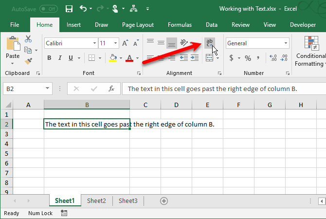
When you enter text in a cell that's wider than the cell, the text goes past the right border of the cell by default. But it's easy to have the text wrap to fit the column width. The text wrap adjusts automatically when you change the width of the cell.
To make text wrap in a cell, select the cell and click the Wrap Text button in the Alignment section of the Home tab.
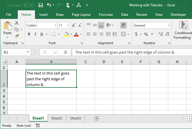
The text is wrapped in the cell and the row height automatically adjusts to fit the text.
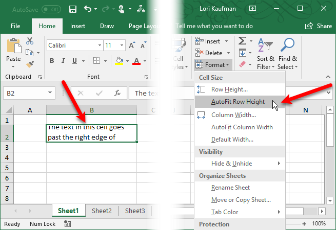
If the row height does not automatically adjust, the row may be set to a specific height.
To automatically fit the row height to the text, select the cell. Then, click Format in the Cells section on the Home tab and select AutoFit Row Height.
If you want to keep the row at a specific height, you can change it to make sure the wrapped text fits. Select Row Height from the Format menu. Then, enter a height for the row on the Row Height dialog box and click OK.
You can also drag the bottom border of the row down until all the lines of text fit in the cell.
Enter a Line Break in a Cell
If the text in a cell goes past the right border, you can also insert a line break to manually make the text wrap.
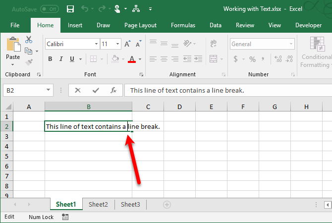
Double-click on the cell to edit the text or press F2. Click the mouse at the point in the text where you want to insert a line break. Then, press Alt + Enter.
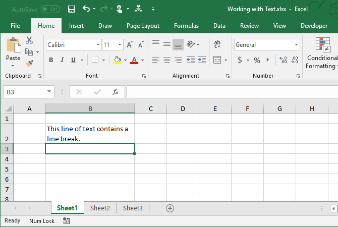
The row height adjusts to fit the text if the Format is set to AutoFit Row Height in the Cells section of the Home tab.
Count Cells Containing Any Text
If you want to know how many cells in a range on your worksheet contains text (not numbers, errors, formulas, or blank cells), you can use the COUNTIF function.
The generic form of the COUNTIF function for counting any number of text characters is:
=COUNTIF(cellrange,"*")
The cellrange represents any range of cells like B2:B9. The asterisk between the quotes is a wildcard character that represents any matching number of text characters. There are a few things to note about what are considered text characters:
- The logical values TRUE and FALSE are not counted as text.
- Numbers that are entered as text are counted in the wildcard character (*).
- A blank cell that begins with an apostrophe (') is counted.
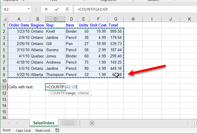
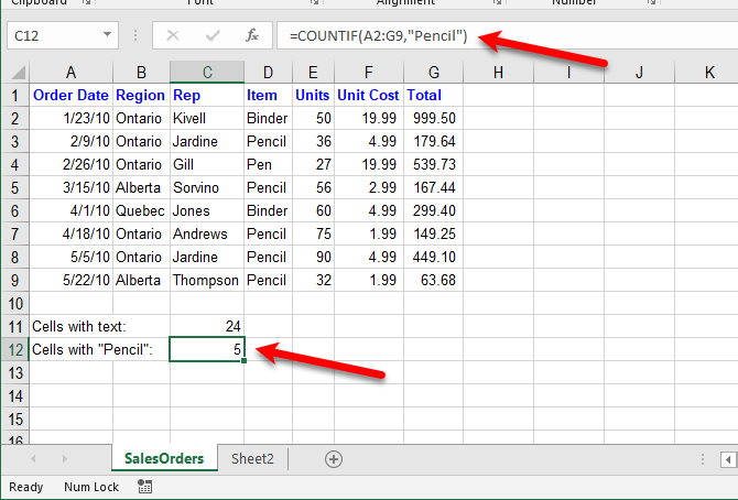
For example, to count the number of cells containing text in the cell range A2:G9 in the following worksheet, we enter "=COUNTIF(". Then, to enter the cell range, we select the cells we want to include in the count.
The COUNTIF function is not case sensitive.
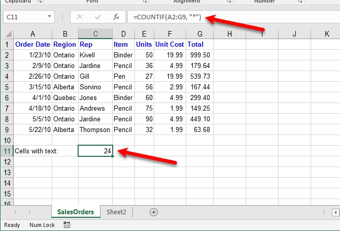
Then, we type a comma (,) and the wildcard character (*) surrounded by double quotes.
Press Enter to complete the function entry and view the result in the cell.
Count Cells Containing Specific Text
You can also use the COUNTIF function to count how many cells contain specific text characters.
The generic function for counting the occurrences of a specific string text characters is:
=COUNTIF(cellrange,"txt")
Just like in the previous section, the cellrange represents any range of cells like B2:B9. We put the string of text characters we want to find between double quotes.
For example, to count the number of cells containing "Pencil" in the cell range A2:G9 on following worksheet, we enter the following function:
=COUNTIF(A2:G9,"Pencil")
This finds all the cells containing just the word "Pencil" with no other text in the cell. Because the COUNTIF function is not case sensitive, it will find all cells containing "Pencil" or "pencil".
The COUNTIFS function allows you to count cells with text but exclude cells with specific text characters.
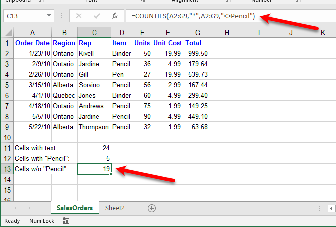
For example, we use COUNTIFS in the following way to find all cells containing any text except for "Pencil".
=COUNTIFS(A2:G9,"*",A2:G9,"<>Pencil")
For the COUNTIFS function, you first give it the range and the text you want to find. Then, give it the same range again and the text you want excluded. The "<>" is used to exclude whatever text follows.
When using either the COUNTIF or COUNTIFS function, you can add an asterisk on one or both sides of the string to find cells that contain that string surrounded by any number of text characters (or none).
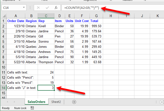
For example, to find all cells containing the letter "j", we use the following function:
=COUNTIF(A2:G9,"*j*")
Again, because the COUNTIF function is not case sensitive, cells containing "j" or "J" will be counted.
Convert Text to Numbers
If you have a lot of cells that contain numbers stored as text, there are a few ways you can convert the text to numbers.
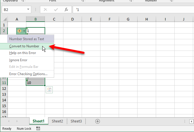
You can tell if a number is formatted as text when it's left-aligned in the cell instead of right-aligned. Also, if a number has been forcefully formatted as text using an apostrophe (') at the beginning, there will be a green triangle in the upper-left corner of the cell.
To convert text to numbers you can use the Convert to Number option, the Text to Columns feature, or Paste Special. We discuss each of these methods in our article about extracting numbers and text in Excel.
Convert a Number to Text
There may be times when you want to store numbers as text. Maybe you're performing an action on a range of cells and there are certain cells you don't want to read as numbers, even though they are.
Typing an apostrophe (') at the beginning of a number converts it to text. But if you have a lot of cells with numbers you want to convert to text, you can use the TEXT function.
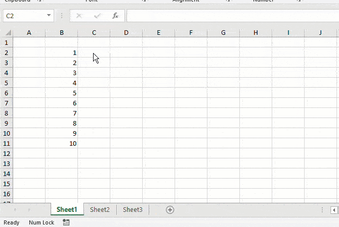
For example, we want to convert the numbers in the B column shown below to text. We type the following function into the cell to the right of the first number.
=TEXT(B2,"0")
You give the function the cell reference for the number to convert and then the number format you want. We're just converting to a number with no special formatting (not currency or a date, for example). So we use "0" (zero).
Use the AutoFill feature to copy the TEXT function to the rest of the cells. The numbers become text and are left-aligned.
You can copy and paste the converted values into the original column. Select the cells containing the TEXT function and press Ctrl + C to copy them. Select the first cell in the original column. On the Home tab, click the arrow on the Paste button and go to Paste Special > Values.
You can find examples of the different text formatting available for use in the TEXT function on Microsoft's support site.
Convert Text to a Date
Have you ever gotten a workbook from someone else in which they entered dates as text, as numbers, or in a format not recognizable as dates? You can convert text to dates using the DATE function.
Here's the generic format of the DATE function:
=DATE(year,month,day)
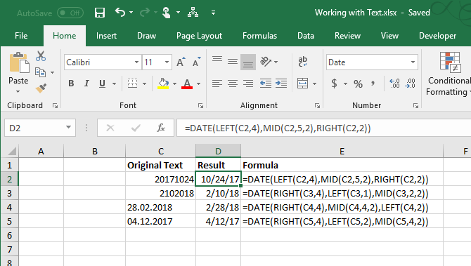
For the year, month, and day, we're going to use the LEFT, MID, and RIGHT string functions to extract the appropriate parts of the text or number we want to convert. We'll explain the four examples in the image below.
To convert "20171024" in cell C2 to a date, we used the LEFT function to extract the first four characters for the year (2017). Then, we used the MID function to extract the two characters starting at the fifth position as the month (10). Finally, we used the RIGHT function to extract the last two characters as the day (24).
=DATE(LEFT(C2,4),MID(C2,5,2),RIGHT(C2,2))
The next example, "2102018" in cell C3, is in a different order. We still use the string functions but in a different order. We used the RIGHT function to extract the last four characters for the year (2018). The month is only one digit in this case, so we used the LEFT function to extract the first character as the month (2). Finally, we used the MID function to extract the two characters starting at the second position as the day (10).
=DATE(RIGHT(C3,4),LEFT(C3,1),MID(C3,2,2))
The dates in cells C4 and C5 look like normal dates, but Excel doesn't recognize them as dates. In cell C4, the format is day, month, year. So we use the RIGHT, MID, and LEFT functions in the following way:
=DATE(RIGHT(C4,4),MID(C4,4,2),LEFT(C4,2))
In cell C5, the format is month, day, and year, using two a zero in front of a single-digit month. So we use the RIGHT, LEFT, and MID functions in the following way:
=DATE(RIGHT(C5,4),LEFT(C5,2),MID(C5,4,2))
Using the DATE function may seem like just as much work as retyping the text as dates. But it's a good likelihood that the same format was used throughout your workbook if one person worked on it.
In that case, you can copy and paste the function and the cell references will adjust to the correct cells. If they don't, simply enter the correct cell references. You can highlight a cell reference in a function and then select the cell you want to enter that reference.
Combine Text From Multiple Cells
If you have a large amount of data on a worksheet and you need to combine text from multiple cells, there's an easy way to do so. You don't have to retype all that text.
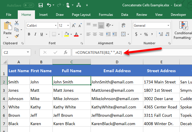
For example, we have a worksheet containing names of employees and their contact information, as shown below. We want to separate the First Name and Last Name and then combine them into a Full Name column. We can also create an Email Address automatically by combining the first and last name.
To do this, we use the CONCATENATE function. To "concatenate" simply means "to combine" or "to join together." This function allows you to combine text from different cells into one cell. You can also add any other text to the text from other cells.
To combine the Last Name and First Name in one row into the Full Name column, we use the CONCATENATE function in the following way:
=CONCATENATE(B2," ",A2)
Give the CONCATENATE function the text to combine in the order you want it put together. So we gave the function the First Name (B2), a space in double quotes (" "), then the Last Name (A2).
We can also build the email address in the same way. We use the First Name (B2), the Last Name (A2), and then the rest of the email address (@email.com) in double quotes.
=CONCATENATE(B2,A2,"@email.com")
Always put any specific text in double quotes, but do not put quotes around cell references.
Separate Text Into Multiple Cells
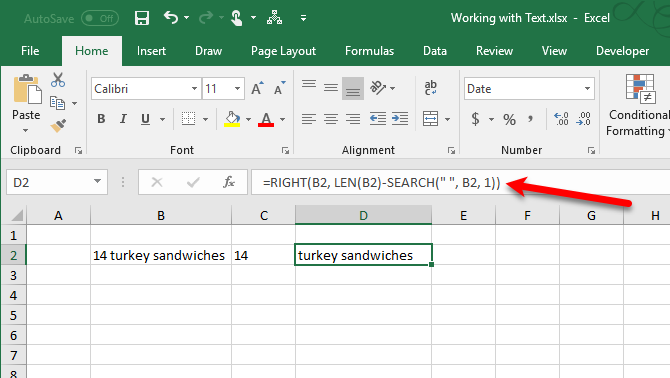
Do you have some cells with mixed format content that you want to separate? For example, if you have a cell containing "14 turkey sandwiches", you can separate that into the number (14) and the text (turkey sandwiches). That way, you can use the number in functions and formulas.
To get the number out of "14 turkey sandwiches", we use the LEFT string function.
=LEFT(B2,SEARCH(" ",B2, 1))
First, we give the function the cell reference for the text from which we want to extract the number (B2). Then, we use the SEARCH function to find the first space after the first character in the string.
To get the text out of "14 turkey sandwiches", we use the RIGHT string function.
=RIGHT(B2,LEN(B2)-SEARCH(" ", B2, 1))
First, we give the RIGHT function the cell reference from which we want to extract the text (B2). Then, we use the LEN and SEARCH functions to determine how many characters in from the right we want to get. We're subtracting the number of characters from the first space after the first character in the string to the end of the string from the total length of the string.
Get more details about separating text into multiple cells in our article about extracting text or numbers from mixed format cells.
More on Working With Text Functions in Excel
Sometimes the spreadsheet you are working on will have too much of text. These will help you simplify it.
You can find more details about the functions we discussed here in our article about text operations, as well as information about some additional related functions we didn't mention here.

