Conditional formatting in spreadsheets is a terrific feature that makes your data stand out. You simply place conditions around the values in a cell or group of cells. When those conditions are met, you can automatically have the cell highlighted, the text formatted, or both. This makes specific data pop.

If you would like to set up conditional formatting in Numbers on Mac, we're here to help. As you follow this tutorial, note that in Numbers, the feature is referred to as conditional highlighting, rather than conditional formatting.

Types of Data for Conditional Highlighting

Before adding a rule for conditional highlighting, here is a list of the types of data you can use and the corresponding conditions.

• Numbers: Equal to, not equal to, greater than, greater than or equal to, less than, less than or equal to, between, and not between
• Text: Is, is not, starts with, ends with, contains, and does not contain
• Dates: Yesterday, today, tomorrow, in this, in the next, in the last, exactly, before, after, between, the date, before the date, after the date, and in the range
• Durations: Same options as Numbers
• Blank: Is blank or is not blank

For additional ways to view your data, you might also take a look at using interactive charts and graphs in Numbers.

Set Up a Conditional Highlighting Rule for Numbers

Numbers are the most popular types of data you will use in spreadsheets. Whether a simple number, money, or percentage, numbers are everywhere in spreadsheets.

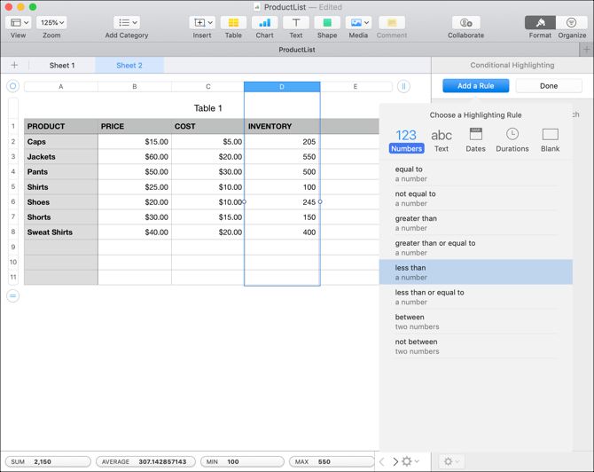
For setting up conditional highlighting surrounding numbers, we're going to use a product sheet as an example. This data includes numbers for price, cost, and inventory, but we'll concentrate on inventory.

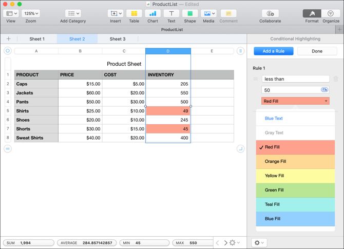
Let's say you want to quickly see when inventory for a product falls below a certain amount. For instance, 50. We'll have Numbers highlight those cells in red. Here's how to set this up.

1. Select the cells in your spreadsheet. You can select a group by clicking the first one and dragging through the rest or select an entire column or row.
2. Click the Format button on the top right to open the sidebar if it's closed.
3. Select Cell from the top of the sidebar.
4. Click the Conditional Highlighting
5. Click Add a Rule.
6. Select Numbers and then Less than.

Now you can customize your rule in the sidebar to apply the formatting. Enter the number (50) in the box under your condition (less than) and then select your formatting from the dropdown box (Red Fill). You should see the changes immediately if you have values that meet the condition. Click Done.

Set Up a Conditional Highlighting Rule for Text

Text is another widely-used data type in spreadsheets. And for teachers or professors who use Numbers for tracking students' grades, conditional highlighting is super handy.

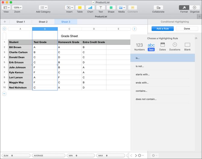
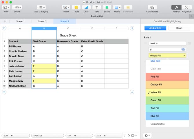
So, for this example, we'll use a grade sheet. Let's say that whenever a student receives an F on a test, we want to highlight that grade in yellow so we can offer them extra credit. Here's how to set this up.

1. Select the cells in your spreadsheet.
2. Click the Format button on the top right to open the sidebar if it's closed.
3. Select Cell from the top of the sidebar.
4. Click the Conditional Highlighting
5. Click Add a Rule.
6. Select Text and then Is.

Next, customize your rule in the sidebar. Enter the text (F) in the box under your condition (text is) and then select your formatting in the dropdown box (Yellow Fill). Once again, you'll see the changes right away for values that meet the condition. Click Done.

Set Up a Conditional Highlighting Rule for Dates

Using dates in spreadsheets is ideal for so many business and personal situations. From employee records to household budgets to project management, you probably have dates in a spreadsheet already.

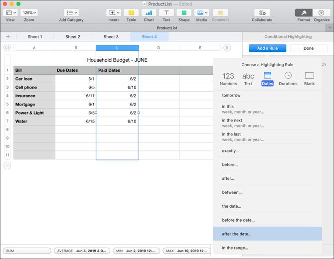
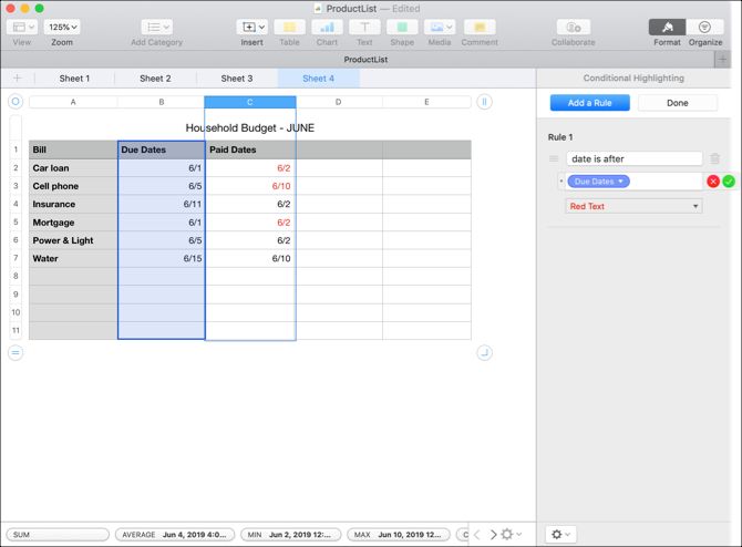
One of the best ways to use conditional formatting for dates is to make past due dates for bills stand out. So, this is our next example. We'll set up a rule for all Paid Dates that are past the Due Dates to display in red text.

Here's how to set up conditional highlighting for dates that come after other dates.

1. Select the cells in your spreadsheet.
2. Click the Format button on the top right to open the sidebar if it's closed.
3. Select Cell from the top of the sidebar.
4. Click the Conditional Highlighting
5. Click Add a Rule.
6. Select Dates and then After the date.

To set this rule up easily, instead of entering a value in the box under the condition, like a number or text, we are going to select the cells.

Click the button inside of the box where you would enter a condition value. Then, select the cells that contain the dates. Next, click the checkmark. Now you can see that all Paid Dates that are after the Due Dates have red text. Click Done.

Set Up a Conditional Highlighting Rule for Durations

Durations might not be the most popular types of data entries in Numbers, but if you manage projects or track tasks, durations are handy. And highlighting certain durations is even handier.

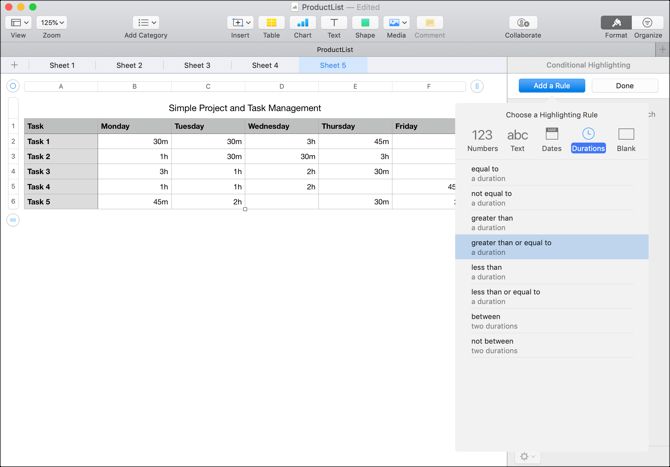
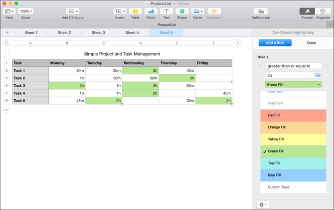
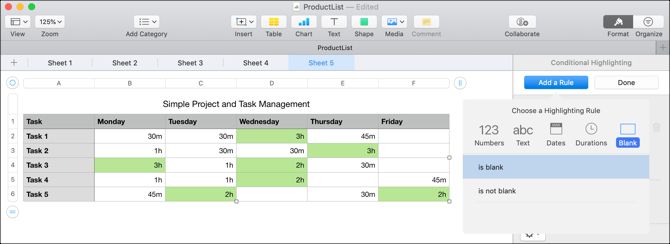
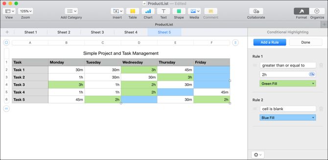
For this example, we're going to use a simple project management task sheet. Here, we track the time we spend on tasks each week. Now, we want to see those days where we spent two or more hours on a single task highlighted in green. Here's how to set this up.

1. Select the cells in your spreadsheet.
2. Click the Format button on the top right to open the sidebar if it's closed.
3. Select Cell from the top of the sidebar.
4. Click the Conditional Highlighting
5. Click Add a Rule.
6. Select Durations and then Greater than or equal to.

Now, customize your rule. Enter the duration (2h) in the box under your condition (greater than or equal to) and then select your formatting in the dropdown box (Green Fill). Click Done.

Set Up a Conditional Highlighting Rule for Blanks

One more convenient highlighting rule to set up in Numbers is for blank cells. You could use this in each of our examples above like missing inventory counts, student grades, and dates for bills.

To show you how to set up this rule, we'll use our project management spreadsheet and have all blank durations display in blue.

1. Select the cells in your spreadsheet.
2. Click the Format button on the top right to open the sidebar if it's closed.
3. Select Cell from the top of the sidebar.
4. Click the Conditional Highlighting
5. Click Add a Rule.
6. Select Blank and then Is blank.

Next, just select the highlighting type from the dropdown box since there is no value to add under the condition. Click Done.

Create Your Own Custom Style for Highlighting

While the basic formatting options are fine, like bold text or colored cells, maybe you want something more specific. Great news, you can make your own custom style!

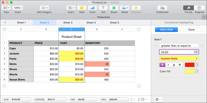
To create your own style, set up your conditional highlighting rule using the steps above. When you get to the part where you pick the formatting from the dropdown box, go all the way to the bottom of the box and click Custom Style.

You can then format the text with bold, italics, underline, or strikethrough. And you can use color for the text in addition to a color for the cell. So, this lets you combine all sorts of formatting that suits your needs best.

In our example below, for all project costs that are $20 or more, our cells are formatted with yellow highlight and red text that's also bold.

Take Advantage of Conditional Formatting in Numbers on Mac

Hopefully, this tutorial will get you off to a great start in using conditional highlighting in Numbers on your Mac. Learning how to use formulas and functions in Numbers is also handy for analyzing data.

For more help with Numbers, find out how to find and remove duplicate values.