
Record a task, save that task, and run the task whenever you want.
Macros are finally available to Google Sheets users. Macros allow you to automate repetitive tasks in documents and spreadsheets without having to learn to write code.
They have been a core productivity tool in Microsoft Office for a long time. Excel users have long been able to use macros to save time and now you can bring the same time-saving benefits to Google Sheets.
While Google Sheets has long allowed users to write their own Apps Script functions, macros open up this kind of functionality to all Google Sheets users---no coding experience required.
Macros are particularly useful if you find yourself dealing with multiple sheets over and over with similar data or information. For instance, any kind of monthly trackers with elaborate functions to collate data will benefit from the of macros.
How to Create a New Macro in Google Sheets
Google Sheets macros are remarkably easy to create.
- Click Tools > Macros > Record Macro.
- Run through the steps you want to automate.
-
Choose Absolute References if you want the macro to operate in the exact same cell you record. Choose Relative References if you want the macro to operate in the cell you select and nearby cells.
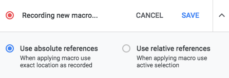
- Click Save.
- Enter the name of the macro and an optional keyboard shortcut key.

Now obviously, step two in the list above could involve a lot more steps, but more on that later.
How to Edit a Macro in Google Sheets
If you want to edit your Macro, do the following:
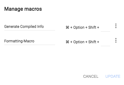
- Go to Tools > Macros > Manage Macros.
-
In the list of Macros that opens up, click the menu button (three dots) next to the macro you want to edit.
- Click Edit Script.

To edit the macro, you're going to have to actually edit the code, so if this is something you're not comfortable with, it may be easier to simply re-record the macro.
How to Run a Macro in Google Sheets
To run the macro, open the sheet you want to use it, and click Tools > Macros and select the macro from the list. Or if you assigned a keyboard shortcut to your macro, you can use that instead.

Below, you'll find a few simple examples of the various ways you can use macros in Google Sheets.
Example 1: Format Your Spreadsheet With a Macro
Any sort of repetitive formatting that you have to apply to several Google sheets can easily be done with macros.
Basic Formatting
If you have multiple sheets with similar information, you can record macros for any or all of the following: bold/italic/underline formatting, font size, text alignment, text wrapping, background fill color, and more.

Conditional Formatting
With Google Sheets, you can also get pretty meta, by adding an extra layer of automation on top of basic automation with Conditional Formatting.
You can use Conditional Formatting to format cells using the same methods listed above. The difference is that you can create a rule that formats the text based on specific criteria:
- If the cell contains or does not contain a specific keyword.
- If the cell contains a number equal to, greater than, or less than a specific number
- If the cell contains a specific date/a date after/a date before your specification.
So let's say you're using Google Sheets as a way to keep track of your tasks, and have assigned due dates to your tasks. You can use conditional formatting to highlight anything that is due today:
- After clicking Record, select the cells you want to apply conditional formatting to.
- Go to Format > Conditional Formatting.
- In the sidebar that opens, click Add new rule.
- Under Format Cells if select Date is.
- In the second dropdown menu that opens, select Today for tasks due today.
If you want to highlight anything that is past due, repeat steps 1 to 3 and then do the following:
- Under Format Cells if select Date is before.
- In the second dropdown menu that opens, select Today.
Example 2: Create Reports and Charts
There are plenty of ways you can generate reports in Google Sheets including Pivot tables, graphs, and charts.
Pivot Tables in Google Sheets
Pivot Tables are extremely useful if you're looking to calculate totals of various items in your spreadsheet. You can use a Pivot Table to understand large amounts of data and summarize it into a brief digestible report. Since it is based on the spreadsheet data, you can use conditional formatting, charts, and graphs to visualize the data too.
For instance, if you're using a Google Sheet for your spending habits, you can use a pivot chart to calculate totals. This is a great way to really get a handle on just how much you're spending at Starbucks.
- After clicking Record, go to Data > Pivot Table.
-
The Pivot Table Editor will open up in a side panel where you can add the items you want to that appear in your table.
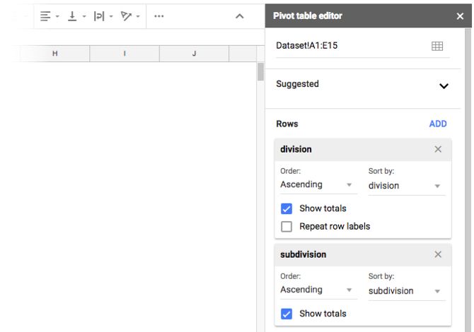
- Under Rows click Add, and select the column containing the information you want to collate: expense category or location for example.
- Under Values, click Add and select the column containing the amounts you're spending per category.

This is a very simple example of how a pivot table can be used. There are far more elaborate uses, where macros will make life much easier for you in Google Sheets.
Graphs and Pie Charts in Google Sheets
Rather than scroll through row upon row of data, you can also summarize all of that information visually.

Again, if you have multiple sheets with similar data, you can create the same chart across several different sheets.
For example, if you're tracking your monthly sales, you could create a pie chart that breaks down sales by product.
- Select the column(s)/row(s) containing the data you want to visualize.
- After clicking the Record button, go to Insert > Chart.
- In the panel that opens up, select the chart type (Line chart, bar chart, pie chart etc.)
Run that macro on other sheets with similar data for quick visualizations. Google Sheets will also make suggestions for the most suitable chart based on the data.
Example 3: Run Complex Functions With Macros
This is probably one of the most useful and powerful ways you can use macros in Google Sheets---but while complex functions can be complicated, they're made simple with macros.
There are plenty of existing functions such as the COUNTIF formula or the Lookup Functions. You can also can take it a step further and create your own Google Sheets functions.
Once you have your function figured out, just record your macro running through the steps.
Example 4: Make Your Data Easier to View

If you have a large amount of data saved in a Google spreadsheet, it helps to freeze the first row and first column.
That way when you're looking at a spreadsheet full of numbers or information, keeping the first row or column in view is essential if you want context for what you're looking for.
- After clicking the Record button, go to View > Freeze > One Row and View > Freeze > One Column.
- Click Save.
- Enter a name for the macro and click Save again.
Start a Macro and Stop Repetitive Work
Because of the collaborative nature of Google Sheets, you can run macros while other people are continuing to enter their information, and no longer have to download sheets and open them up in another program to run a macro.
If collaboration and cloud storage isn't a priority for you, you can always opt for Microsoft Excel to record macros.s