You can use the MAX function to find the largest value in a range. But what if you need to find the 5th, 10th, 4th, 2nd, etc., largest value in a spreadsheet? That’s where the LARGE function comes in. This guide will cover how it works and some practical examples.
LARGE Function Syntax
The LARGE formula is used to find the value for the nth largest value in a dataset, which the user will define. The function is easy to use and doesn't require advanced Google Sheets knowledge. Before we look at examples of how you can use this formula, let’s look at how it works.
Here is the syntax for the LARGE formula in Google Sheets:
=LARGE(dataset, number)
The formula uses two parameters. The first parameter is the dataset used to define an array or a cell range that contains the data you want to search through. The second parameter is the number used to define the rank of the largest number to return. For example, using 6 as the number parameter means that the function will find the 6th largest element in the data set.
How to Use the LARGE Function in Google Sheets
Here are three ways to use the LARGE function within ranges or arrays:
1. In a One Dimensional Array
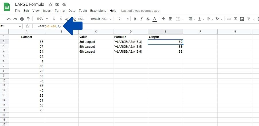
In this example, we have a one-dimensional array that contains 15 values. We want to find the data set's 3rd, 5th, and 6th largest values for this demonstration. Let's look at how you can do this in a spreadsheet. Follow along with the steps below:
- Click on the cell where you would like to add the formula.
- Add an equal (=) sign to start off the formula.
- Add the initial part of the formula, which is LARGE(.
- For the first parameter, we enter the dataset. In this case, it is A2:A16.
- Add a comma (,) to separate the parameters.
- Now we will add the number parameter, which in this example are 3, 5, and 6, respectively in each cell.
- Add a closing bracket to finish the formula.
- Press Enter.
Google Sheets will now go through the data and find the nth number value of the largest number in the data set.
2. In a Two-Dimensional Array
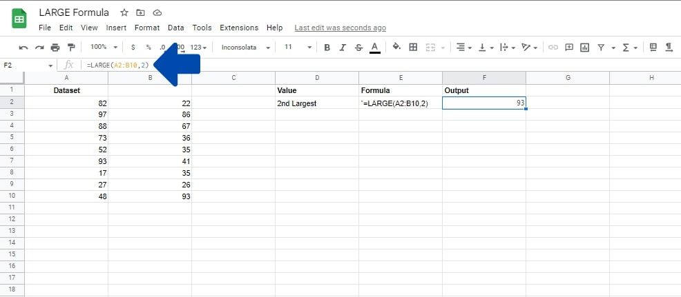
Below, we have a two-dimensional array that contains 18 values. For this demonstration, we want to find the 2nd largest value in the data set. Let us look at how you can do this in your spreadsheet.
It works similarly to the first example; only you have to add values that spread over several columns as the dataset argument. Here are the steps you would need to follow:
- Click on the cell where you would like to add the formula.
- Add an equal (=) sign to start off the formula.
- Add the initial part of the formula, which is LARGE(.
- Now, for the first parameter, we enter the dataset parameter. In this case, it is the array A2:B10.
- Add a comma (,) to separate the parameters.
- Now we will add the number parameter, which in this example 2.
- Add a closing bracket.
- Press Enter.
3. Using Single Cell Array Literals
Often, you won’t want to display the data in a table in Google Sheets, but you may still want to find the nth largest number in a data set. The LARGE function can also be used with single cells array literals in Google Sheets. This allows you to add and delete the values in the specified array. This means you won't have to execute the formula repeatedly. Rather, you can simply edit the values, and the formula will do the calculations automatically.
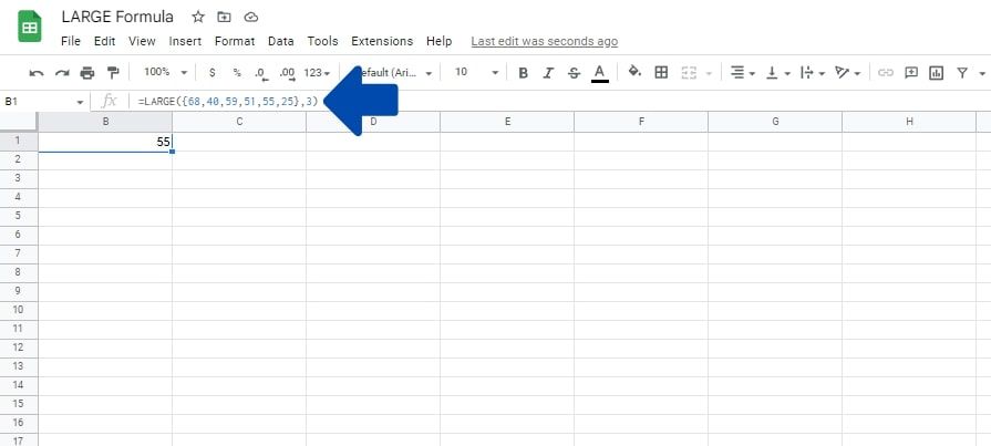
The example below shows six random numbers in a single cell array. We want to find the 3rd largest value in this dataset. Here are the steps you would need to follow to use LARGE in your spreadsheet for this type of calculation:
- Click on the cell where you would like to add the formula.
- Add an equal (=) sign to start the formula and add the initial part of the formula, which is LARGE(.
- For the first parameter, we will enter the array literal. To do this, add an opening curly bracket “{”
- Type in the values for the array literal. In our example, we have 68,40,59,51,55,25 with commas separating each array value.
- Now add a closing curly bracket “}” to finish the array.
- Add a comma (,) to separate the parameters.
- Now we will add the number parameter, which in this example is 3 for the 3rd largest.
- Add a closing bracket
- Press Enter.
You can also apply the LARGE function as part of an ARRAYFORMULA in Google Sheets.
Things to Know About the LARGE Function
- The LARGE formula will ignore FALSE and TRUE values.
- Text values in the range may cause the LARGE function to return an error.
- The value for the number parameter should be lower than the total number of cells in the data set. If the number parameter is higher, the formula will give a #NUM! error.
When Not to Use LARGE in Google Sheets
If text values are in the range, it can break the formula, so you could be better off using MAX instead.
Another situation where you should not use LARGE is when attempting to determine the median of an even range of values. The median is the midpoint of a set of numbers and is an important part of calculating standard deviation in Google Sheets. But when it is calculated with the LARGE function, you need to put the central position as the number argument.
For example, you need to use 3 as the number argument in a set of 5 numbers to find the median with the LARGE function. There is no central number in a data set with an even amount of numbers, and the median would be the average of the two central numbers. Instead, you should use the MEDIAN function.
Formulas That Are Similar to LARGE in Google Sheets
Here are a few similar functions that should come easy now that you’ve learned about LARGE:
- SMALL: Finds the nth smallest number.
- MIN: Finds the minimum value in a data set.
- MAX: Finds the maximum number in a data set and is often used in place of LARGE.
LARGE vs. MAX Function
With LARGE, you can specify the value's rank, such as first highest, second highest, and so on. The MAX function can return only the first largest element in the range.
The LARGE function returns a "#NUM! error" when applied to a range of only text values. However, regardless of the values in the range, you can still use the MAX function. MAX will return 0 if the range contains only text values.
A LARGE Amount of Learning
Although using LARGE on its own is pretty straightforward, functions in Google Sheets are often combined to make more complex formulas. It’s a good idea to familiarize yourself with as many functions as possible, so you can tackle these more difficult spreadsheet problems.


