
Figuring out actionable insight is the primary goal for any database. Microsoft Excel offers the VLOOKUP and HLOOKUP functions to find data from a large spreadsheet. However, these functions aren’t flexible enough.
You can use INDEX and MATCH in Excel to make your data discovery task easier. You’ll enjoy worry-free data retrieval, even in advanced and complex situations. This article helps you understand these two functions in simple terms and easy-to-understand examples.
What Is the INDEX Function?
The INDEX function of Microsoft Excel fetches a value from a given cell range. Like a GPS device that finds a location on a map, this function finds a cell value within a cell range.
Whereas for a GPS, you need to input latitude and longitude, for the INDEX function to work, you need to provide a cell range, row number, and column number. Here is the syntax:
=INDEX(array, row_num, [column_num])
You can try these steps to apply the INDEX function in a relevant scenario:
- In a cell, put an Equals Sign and then type INDEX.
- Press Tab and enter the first argument.
-
It should be a cell range followed by a comma.
- Enter a row number where you expect the data, and put a comma.
- The column number isn’t necessary since there’s only one source column.
- Put a parenthesis at the end and press Enter.
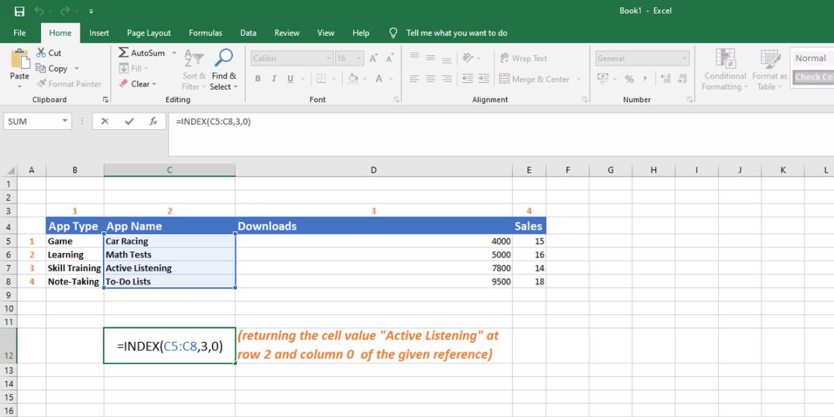
- The formula should look like the following:

=INDEX(C5:C8,3,0)
Download: INDEX and MATCH in Excel tutorial workbook (Free)
What Is the MATCH Function?
If you want to know the row number or column number of a cell value or cell address, you need to use the MATCH function in Excel. It’s helpful when you need to automate a task in Excel, like locating a cell value for the INDEX function.
It requires three inputs to fetch a cell’s position; the lookup value, the cell range where the value exists, and the match criteria. The possible match types are 0 for an exact match, 1 for less than the lookup value, and -1 for greater than the lookup value. Here is the syntax:
=MATCH(lookup_value, lookup_array, [match_type])
Here is how you can try out the MATCH function:
- Enter an Equals Sign in any cell and type MATCH.
-
Press Tab.
- Now select a cell as the lookup reference, or type anything within quotes.
- Select a cell range for source data and then type 0 for an exact match.
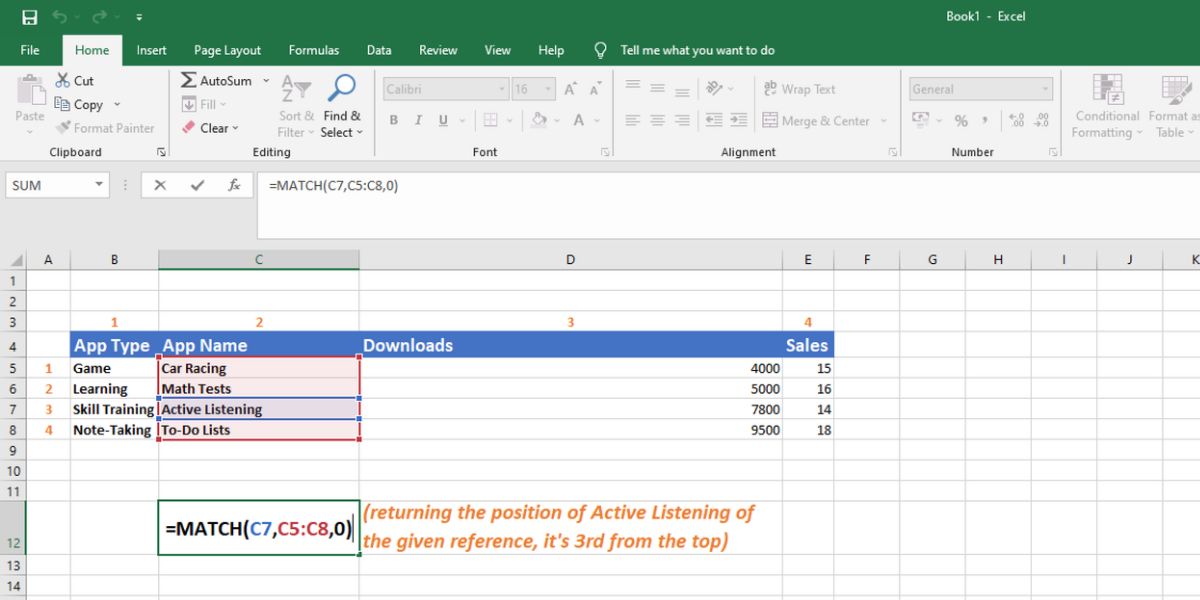
- Press Enter to get the cell position. The following is the formula in action:

=MATCH(C7,C5:C8,0)

            =MATCH("active listening",C5:C8,0)
What Are the Benefits of INDEX and MATCH in Excel?
For complex data lookup tasks, you need to use both functions to unleash their full potential. The benefits of using this formula combination are:
- No restrictions in left to right or right to left lookup
- Easier to delete, insert, or update columns
- For large spreadsheets, the combo formula is much faster than VLOOKUP
- It can fetch approximate matches
- You can create longer nested formulas using these two functions
How to Apply INDEX and MATCH in One Formula
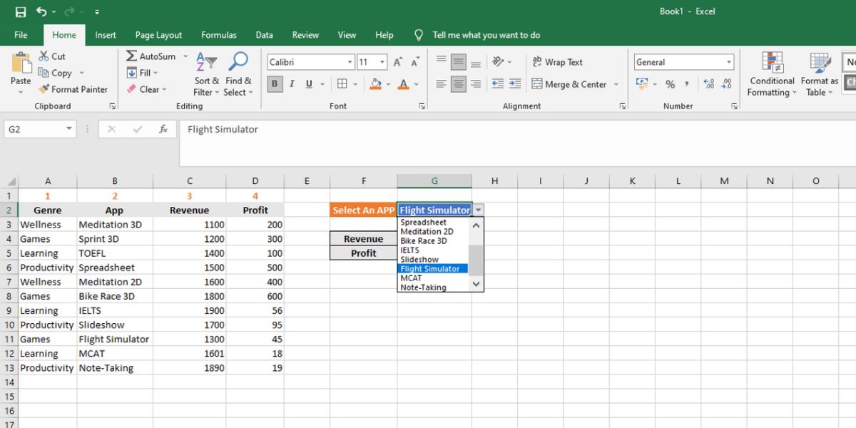
MATCH and INDEX are highly beneficial when you apply them together. Let’s say you want to find out the Revenue and Profit of any app from the given database. Here’s how you can do that:
- Bring up the INDEX function.
-
Select the cells C3:C13 for the Revenue data source.
- Type MATCH and press Tab.
-
Select G2 as the lookup value, B3:B13 as source data, and 0 for a complete match.
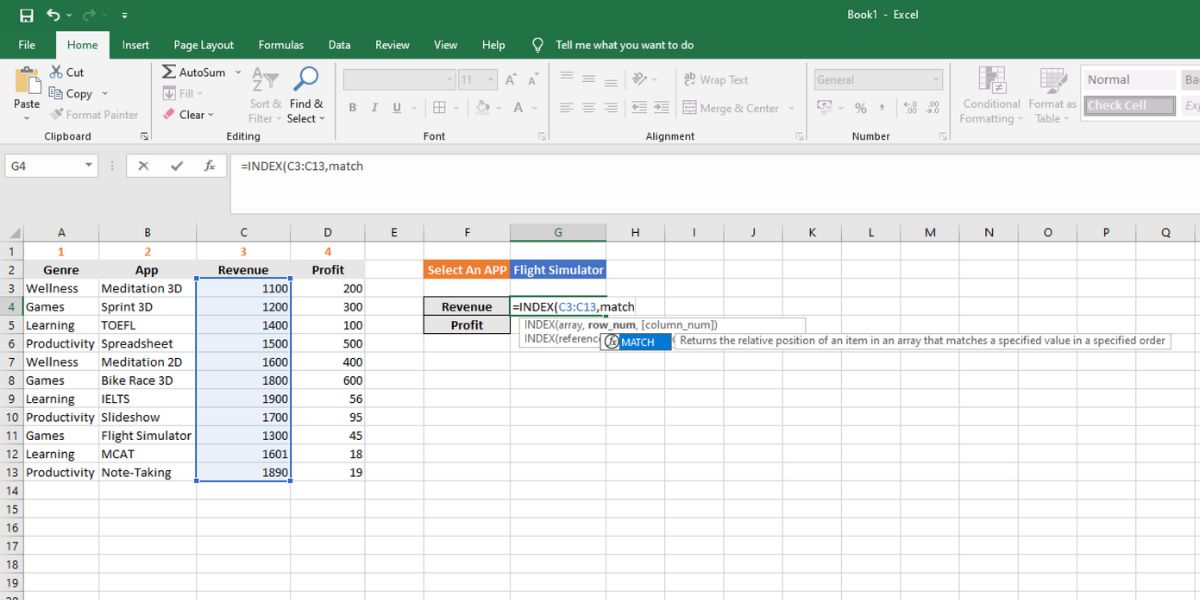
- Hit Enter to fetch the revenue information for the selected app.
-
Follow the same steps and replace the INDEX source with D3:D13 to get Profit.
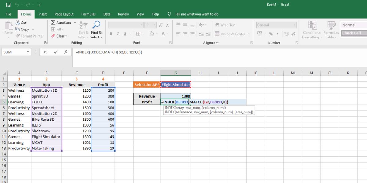
- The following is the working formula:


=INDEX(C3:C13,MATCH(G2,B3:B13,0))

            =INDEX(D3:D13,MATCH(G2,B3:B13,0))
The above-mentioned is an example of the one-dimensional use of INDEX MATCH in Excel. You can also select rows and columns together to execute more complex searches.
For instance, you might want to use a drop-down instead of separate cells for Revenue and Profit. You may follow these steps to practice:
- Select the Revenue cell and click on the Data tab on the ribbon.
-
Click on the Data Validation, and under Allow, select List.
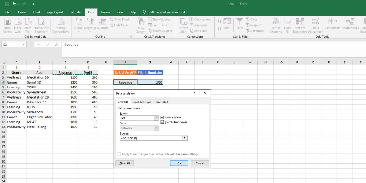
- Select the Revenue and Profit column headers as the Source.
-
Click OK.
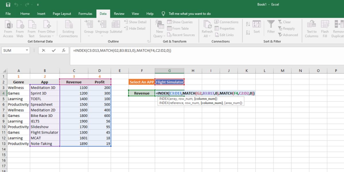
- In this formula, you’ll be using the MATCH function twice to fetch both the row and column value for the final INDEX function.
- Copy-paste the following formula beside the Revenue cell to get values. Just use the drop-down to choose between Revenue and Profit.


=INDEX(C3:D13,MATCH(G2,B3:B13,0),MATCH(F4,C2:D2,0))
In the above formula, the first nested MATCH tells Excel the name of the app for which revenue and profit data is needed. The second one corresponds to the revenue and profit column headers and reflects the relevant values when you swap them in the drop-down menu.
A further complex situation could be looking up data by three column headers, like the name of the app, forecast revenue, and true revenue. Here, you need to use INDEX and MATCH twice to feed each other the inputs they require. You can practice by following these steps:
-
Create three drop-down menus for app name selector, true/forecast, and revenue/profit.
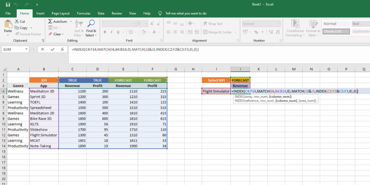
- Now, apply the following formula beside the name of the app where you want the lookup value.

=INDEX(C4:F14,MATCH(I4,B4:B14,0),MATCH(J2&J3,INDEX(C2:F2&C3:F3,0),0))
For both the MATCH and INDEX functions, you can separate multiple inputs for the same arguments by using the & sign. When you need to execute a MATCH function to locate positions of two lookup values, use & between the lookups, and a nested INDEX for a lookup source.
If you notice the second INDEX function, the & sign separates two source arrays. There are no rows or columns, since we need to consider the entire array as possible values.
Looking Up Vital Data Made Easy
Whenever you need to create a dashboard or lookup data from a large matrix, try following the above examples and applying the combined INDEX MATCH formula for convenience. This combo function is more powerful and flexible than the conventional VLOOKUP formula.
You don’t need to worry about the column or row changes since Excel automatically adjusts the selected data source. Hence, you can search more efficiently in your Excel workbook.