Data augmentation is the process of applying various transformations to the training data. It helps increase the diversity of the dataset and prevent overfitting. Overfitting mostly occurs when you have limited data to train your model.
Here, you will learn how to use TensorFlow's data augmentation module to diversify your dataset. This will prevent overfitting by generating new data points that are slightly different from the original data.
The Sample Dataset You Will Use
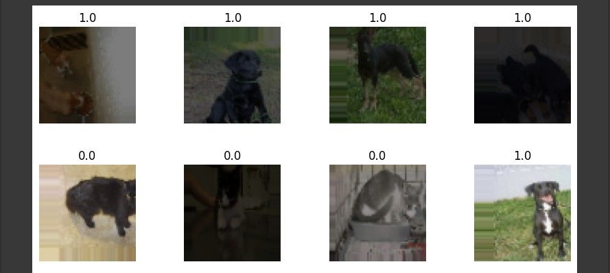
You will use the cats and dogs dataset from Kaggle. This dataset contains approximately 3,000 images of cats and dogs. These images are split into training, testing, and validation sets.
The label 1.0 represents a dog while the label 0.0 represents a cat.
The full source code implementing data augmentation techniques and the one that does not are available in a GitHub repository.
Installing and Importing TensorFlow
To follow through, you should have a basic understanding of Python. You should also have basic knowledge of machine learning. If you require a refresher, you may want to consider following some tutorials on machine learning.
Open Google Colab. Change the runtime type to GPU. Then, execute the following magic command on the first code cell to install TensorFlow into your environment.
!pip install tensorflow
Import TensorFlow and its relevant modules and classes.
        import tensorflow as tf
from tensorflow.keras.preprocessing.image import ImageDataGenerator
from tensorflow.keras.models import Sequential
from tensorflow.keras.layers import Conv2D, MaxPooling2D, Flatten, Dense, Dropout
The tensorflow.keras.preprocessing.image will enable you to perform data augmentation on your dataset.
Creating Instances of the ImageDataGenerator Class
Create an instance of the ImageDataGenerator class for the train data. You will use this object for preprocessing the training data. It will generate batches of augmented image data in real time during model training.
In the task of classifying whether an image is a cat or a dog, you can use the flipping, random width, random height, random brightness, and zooming data augmentation techniques. These techniques will generate new data which contains variations of the original data representing real-world scenarios.
        # define the image data generator for training
train_datagen = ImageDataGenerator(rescale=1./255,
                                   horizontal_flip=True,
                                   width_shift_range=0.2,
                                   height_shift_range=0.2,
                                   brightness_range=[0.2,1.0],
                                   zoom_range=0.2)
Create another instance of the ImageDataGenerator class for the test data. You will need the rescale parameter. It will normalize the pixel values of the test images to match the format used during training.
        # define the image data generator for testing
test_datagen = ImageDataGenerator(rescale=1./255)
Create a final instance of the ImageDataGenerator class for the validation data. Rescale the validation data the same way as the test data.
        # define the image data generator for validation
validation_datagen = ImageDataGenerator(rescale=1./255)
You do not need to apply the other augmentation techniques to the test and validation data. This is because the model uses the test and validation data for evaluation purposes only. They should reflect the original data distribution.
Loading Your Data
Create a DirectoryIterator object from the training directory. It will generate batches of augmented images. Then specify the directory that stores the training data. Resize the images to a fixed size of 64x64 pixels. Specify the number of images that each batch will use. Lastly, specify the type of label to be binary (i.e., cat or dog).
        # defining the training directory
train_data = train_datagen.flow_from_directory(directory=r'/content/drive/MyDrive/cats_and_dogs_filtered/train',
                                               target_size=(64, 64),
                                               batch_size=32,
                                               class_mode='binary')
Create another DirectoryIterator object from the testing directory. Set the parameters to the same values as those of the training data.
        # defining the testing directory
test_data = test_datagen.flow_from_directory(directory='/content/drive/MyDrive/cats_and_dogs_filtered/test',
                                             target_size=(64, 64),
                                             batch_size=32,
                                             class_mode='binary')
Create a final DirectoryIterator object from the validation directory. The parameters remain the same as those of the training and testing data.
        # defining the validation directory
validation_data = validation_datagen.flow_from_directory(directory='/content/drive/MyDrive/cats_and_dogs_filtered/validation',
                                                         target_size=(64, 64),
                                                         batch_size=32,
                                                         class_mode='binary')
The directory iterators do not augment the validation and test datasets.
Defining Your Model
Define the architecture of your neural network. Use a Convolutional Neural Network (CNN). CNNs are designed to recognize patterns and features in images.
        model = Sequential()

# convolutional layer with 32 filters of size 3x3
model.add(Conv2D(32, (3, 3), activation='relu', input_shape=(64, 64, 3)))

# max pooling layer with pool size 2x2
model.add(MaxPooling2D(pool_size=(2, 2)))

# convolutional layer with 64 filters of size 3x3
model.add(Conv2D(64, (3, 3), activation='relu'))

# max pooling layer with pool size 2x2
model.add(MaxPooling2D(pool_size=(2, 2)))

# flatten the output from the convolutional and pooling layers
model.add(Flatten())

# fully connected layer with 128 units and ReLU activation
model.add(Dense(128, activation='relu'))

# randomly drop out 50% of the units to prevent overfitting
model.add(Dropout(0.5))

# output layer with sigmoid activation (binary classification)
model.add(Dense(1, activation='sigmoid'))
Compile the model by using the binary cross-entropy loss function. Binary classification problems commonly use It. For the optimizer, use the Adam optimizer. It is an adaptive learning rate optimization algorithm. Finally, evaluate the model in terms of accuracy.
model.compile(loss='binary_crossentropy', optimizer='adam', metrics=['accuracy'])
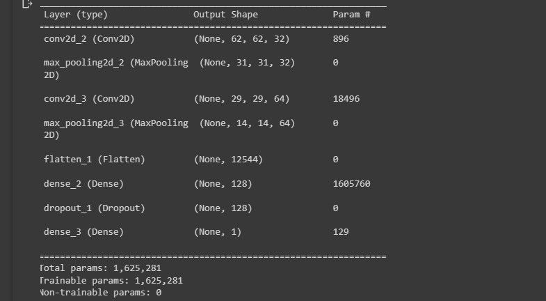
Print a summary of the model's architecture to the console.
model.summary()
The following screenshot shows the visualization of the model architecture.
This gives you an overview of how your model design looks.
Training Your Model
Train the model using the fit() method. Set the number of steps per epoch to be the number of training samples divided by the batch_size. Also, set the validation data and the number of validation steps.
        # Train the model on the training data
history = model.fit(train_data,
                    steps_per_epoch=train_data.n // train_data.batch_size,
                    epochs=50,
                    validation_data=validation_data,
                    validation_steps=validation_data.n // validation_data.batch_size)
The ImageDataGenerator class applies data augmentation to the training data in real time. This makes the training process of the model slower.
Evaluating Your Model
Evaluate the performance of your model on the test data using the evaluate() method. Also, print the test loss and accuracy to the console.
        test_loss, test_acc = model.evaluate(test_data,
                                     steps=test_data.n // test_data.batch_size)
print(f'Test loss: {test_loss}')
print(f'Test accuracy: {test_acc}')
The following screenshot shows the model's performance.
The model performs reasonably well on never seen data.
When you run code that does not implement the data augmentation techniques, the model training accuracy is 1. Which means it overfits. It also performs poorly on data it has never seen before. This is because it learns the peculiarities of the dataset.
When Is Data Augmentation Not Helpful?
- When the dataset is already diverse and large: Data augmentation increases the size and diversity of a dataset. If the dataset is already large and diverse, data augmentation will not be useful.
- When the dataset is too small: Data augmentation cannot create new features that are not present in the original dataset. Therefore, it cannot compensate for a small dataset lacking most features that the model requires to learn.
- When the type of data augmentation is inappropriate: For example, rotating images may not be helpful where the orientation of the objects is important.
What Is TensorFlow Capable Of
TensorFlow is a diverse and powerful library. It is capable of training complex deep learning models and can run on a range of devices from smartphones to clusters of servers. It has helped power edge computing devices that utilize machine learning.


