
Data Validation in Excel allows you to control what the users can enter in a cell. Learn to use Data Validation and even create a drop-down list with it.
What Is Data Validation in Excel?
The Data Validation feature in Excel allows you to specify what kind of data the user may enter in a cell. With Data Validation, you can create a drop-down list of your values for the user to choose from, or set a minimum and maximum value for the data they can enter, and much more.
Data Validation in Excel also allows you to display alerts and input messages to inform the user of what they can enter in a given cell. Data Validation is simple in nature, but you can also use it to validate user-input with your own custom formulas.
How to Use Data Validation in Excel
The basic of using Data Validation is that you select the cell(s) you want to validate data for, and then create a Data Validation rule for them. To bring up the Data Validation dialogue:
- Select your cell(s).
- From the Ribbon, go to the Data tab.
- Click on Data Validation.
Microsoft Excel offers plenty of options to choose from, so before we start, let's have a quick glance at what you'll be working with.
Choosing From the Data Types
In the Data Validation dialogue, the first tab is labeled Settings and contains the validation criteria. This is where you'll be creating the data validation rule.
You can control what kind of data your cell will be accepting by choosing it from the drop-down list under Allow.
Microsoft Excel offers plenty for you to choose from (such as date, time, text, whole number, list, and more). However, you can also use your own formula by selecting Custom from the drop-down list.

The second part of the Settings tab is defining extremums and deciding how the Data Validation rule should behave regarding this extremum.
For instance, after selecting between, you can select a minimum and maximum, and if the user enters invalid data, Excel won't accept it.
Adding an Input Message
You can add an Input Message to inform the user of the Data Validation rules with a custom message when they select the cell. Adding an input message is optional, but it's good practice to add one so that the user knows what the cell is anticipating.

Creating an Error Alert
In the Error Alert tab, you decide how the data validation rule is imposed. There are three alert styles you can choose from. These styles also have different functions:
Stop: This alert style prevents the user from entering invalid data in the cell. The user can attempt again and enter valid data.
Warning: This alert style warns the user that the data they entered is invalid, but still allows them to enter it. The alert window offers three choices to the user: Yes (to enter the invalid data), No (to edit the invalid data), and Cancel (to delete the invalid data).
Information: Much like the Warning alert style, the Information alert style doesn't do anything to keep the user from entering invalid data and only informs them. This alert style offers two choices to the user: OK (to enter the invalid data) and Cancel (to delete the invalid data).

You can also entirely disable the alert by unchecking Show error alert after invalid data is entered option. Doing this, however, undermines the whole point of data validation, since the Data Validation rule will exist but won't enforce in any way.
Data Validation Example: Creating a Drop-Down List in Excel
Now to put together everything you've learned, let's use Data Validation to create a drop-down list.
Drop-down lists are an excellent way for forcing the users to select an item from a list you provide them with, rather than entering their own values.
This increases the data entry speed and also reduces the chances of user-made mistakes in data entry. You can create drop-down lists with Data Validation.
Drop-down lists are different from custom lists. You can use custom lists in Excel to store data you use often. If you want to learn more about custom lists, read our article on how to create a custom list in Excel.
For this example, let's say we have a list of student names, and we're going to choose their courses from a drop-down list. First things first, let's create a table of names:
- Select cell A1 and type "NAME".
- In the cells below, add a bunch of names.
-
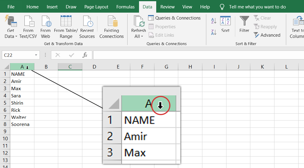
Hover your cursor under the column header (i.e. A) and click it when the cursor becomes an arrow. This will select the entire column.
- Go to the Insert tab and then click on Table.
- Check My Table Has Headers and then click OK. This option will list the top cell (i.e. NAME) as the table header.

Next up, let's create a table for courses where the user will be able to select a course for each student.
- Select cell B1 and type "COURSE".
- Select the entire column by clicking right under the column name (same as the previous table).
- Go to the Insert tab and then select Table to create a table.
- Check My Table Has Headers and then click OK.

Now that you have the table for courses, it's time to provide a list of courses.
- Click the plus sign next to Sheet1 to create a new sheet.
- In the new sheet, type the name of the courses in a column.
Finally, let's use Data Validation to create a drop-down list of the courses.
- Select the cells in the COURSE column.
- Go to the Data tab and then click on Data Validation.
- In the Settings tab, under Allow, choose List.
- Click the Source box.
- Go to Sheet2 and select the cells containing the course names (A1:A5 in this example).
So far, you've created the Data Validation rule. If you want to do this thoroughly, you should add an input message as well.
- In the Data Validation window, Go to the Input Message tab.
- Type in a title and then a custom message.

Finally, let's enforce this Data Validation rule. Even though we've provided a list for the users to choose data from, it's still possible to type other data into the cell. To prohibit this, you should create an Error Alert.
- In the Data Validation window, go to the Error Alert tab.
- Set the Style to Stop. By doing this, the user will only be able to enter what's in the list.
- Type in a Title and then enter an Error Message. You can also leave these blank.
- When you're all set, click OK in the Data Validation window.

That's it! Go ahead and check out your results. Click the cell in front of each name and watch the drop-down list you just created. Or try entering invalid data to get hit with the Error Alert.


There are various approaches to creating a drop-down list. For a more in-depth guide, read our article on dropdown lists in Excel.
Control The Data In Your Excel Document
Now that you have learned the basics of Data Validation, you can maximize accuracy in data input from your users or simplify data entry with a drop-down list. You've learned to utilize a useful Excel feature, but there's still much more to learn.