Being an Excel user, you might be aware of the average function. Generally, it takes the sum of all the values and divides them by the number of values. But let’s say you don’t want to take the average of all values, but only some specific ones.
If that’s the case you’re in, it’s best to find an alternate function in Excel that makes this possible. This is where AVERAGEIF function in Excel comes into play.
The AVERAGEIF function in Excel returns the average of cells if they meet certain criteria. The criteria can be applied to data types like dates, numerical values, and text. In this article, we will go through AVERAGEIF and its examples.
What Is the AVERAGEIF Function in Excel?
As mentioned above, Excel's AVERAGE function gives you the AVERAGE of the values in a range of cells if they meet your specified criteria. Here are the Syntax and Arguments for the AVERAGEIF function.
Syntax
=AVERAGEIF(range, criteria, [average_range])
Arguments
- Range: The range of cells that you want to be assessed by this function.
- Criteria: The criteria that decide which cells are taken into consideration for averaging.
- sum range (optional): The range of cells that needs to be averaged together. If you get rid of it, the cells in the range are averaged collectively.
How to Use the AVERAGEIF Function in Excel
Using the AVERAGEIF function is quite similar to using the SUMIF functions in the cells. To use AVERAGEIF, you simply need to click on the cell where you want the function, and type the syntax of the AVERAGEIF function.
Alternatively, you can also use the “Formula bar” box located on the top of columns after selecting the cell; and insert the syntax of the AVERAGEIF function. Using AVERAGEIF function is comparatively easier, and you wouldn’t need a learning curve as well. You might find it difficult at first, but it is actually quite easy.
Pros and Cons of Using AVERAGEIF Function in Excel
While the AVERAGEIF function is a time-saver, it has its own advantages and disadvantages. Let’s discuss some Pros and Cons of the AVERAGEIF function.
Pros
- Easier to learn and implement.
- Adds the ability to use logical operators.
- Adds flexibility for adding dates into the argument criteria.
Cons
- An error occurs when no cell in the range meets the criteria or the range is blank.
- If the criteria is not specified, the AVERAGEIF function treats the result as 0.
- Ignore cells with the values TRUE or FALSE.
Examples of Using AVERAGEIF Function in Excel
The AVERAGEIF function is a little different from what you expect. In many ways, it is quite similar to the SUMIF function, but there is just one additional step. Let's take an example, so you can understand it better.
Numerical Criteria Example
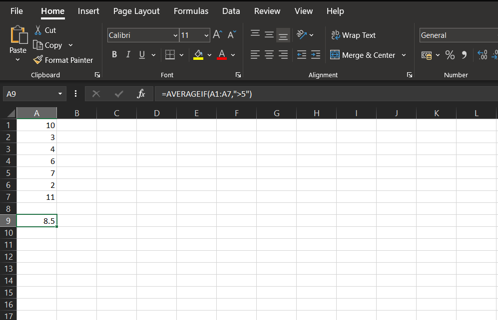
Let’s take a spreadsheet with simple values to explain the potential of the AVERAGEIF function. Assume the values shown in the image below. Suppose we want the average of values that are more than 5 in the range A1:A7.
In such a case, we would select the resultant cell (A9 in our case), and write the condition =AVERAGEIF(A1:A7,”>5”). In our case, the values in A1 to A7 cells are 10, 3, 4, 6, 7, 2, 11. Once we apply the AVERAGEIF function, the result would take an average of 10, 6, 7, 11. The result, as expected, is 8.5 in the A9 cell.
Text Criteria Example #1
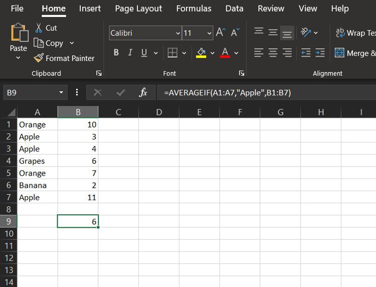
Let’s take a spreadsheet with simple values to explain the potential of the AVERAGEIF function in text scenarios. Assume the values as shown in the image below. In this case, let us suppose you want to consider the values with the text Apple in the A1 to A7 range.
Now we have values from the B1 to B7 range that needs to be averaged. Also, let us get the result of the average in the B9 cell. In such a case, we will now use the condition: =AVERAGEIF(A1:A7,”Apple”.B1:B7).
In our case, the result would take A2, A3, and A7 cells; then average the corresponding cells, which are B2, B3, and B7. As a result, we would get the result in the B9 cell as 6.
Text Criteria Example #2
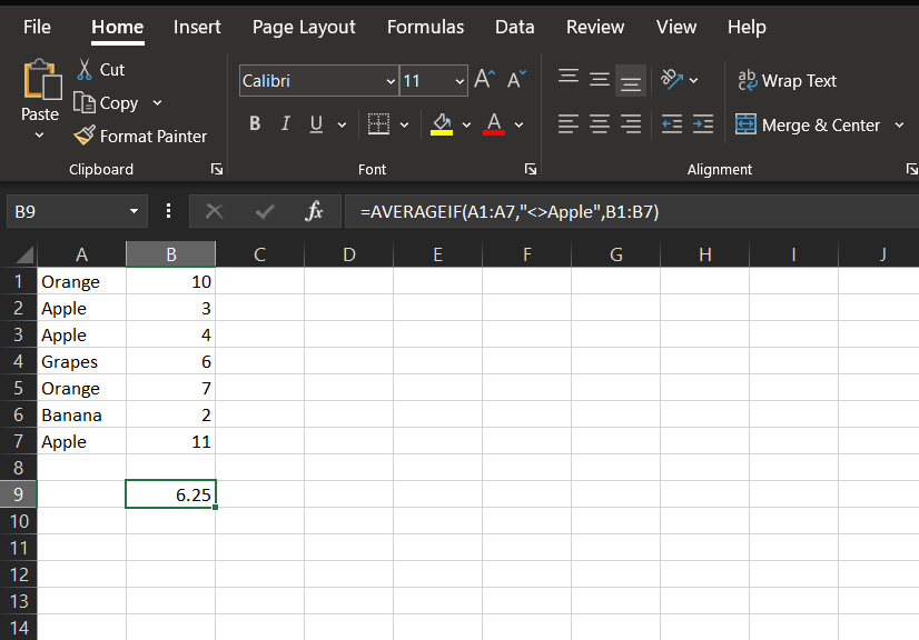
Let’s take the same spreadsheet that we used in Text Example #1, and instead of taking the values corresponding to the text “Apple,” we would take the values that don’t correspond to the text “Apple.”
So in our case, the condition will be =AVERAGEIF(A1:A7,"<>Apple",B1:B7). So it’ll take the A1, A4, A5, A6 cells, instead of the A2, A3, and A7 cells. As a result of this, we would see the average of the cells B1, B4, B5, and B6 cells. In the end, the B9 cell gives the average of 10, 6, 7, and 2, which would be 6.25.
Date Criteria Example
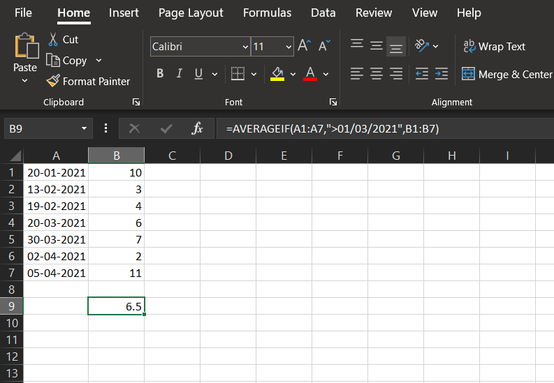
The date criteria is another way to utilize Excel's AVERAGEIF function, similar to that of the numerical and text criteria. Let’s take an example of the spreadsheet that includes the date next to some corresponding values.
In this case, we have some dates in the A1 to A7 range of cells, and some corresponding values. Suppose you want to have the average of values next to dates after 01st March 2021, then the condition would be =AVERAGEIF(A1:A7,">01/03/2021",B1:B7).
The condition would take the cells A4, A5, A6, A7 cells, and average the cells next to them. So the values would be taken as 6, 7, 2, and 11. The average of these values are displayed in the B9 cell, which is 6.5.
Using AVERAGEIF Function Is Simple in Excel
The AVERAGEIF function can be used in multiple scenarios, as we mentioned above. You can treat the AVERAGEIF function as an enhanced version of the simple AVERAGE function in Excel.
When you want to average only certain values in a long range of cells, you can’t look at each cell one-by-one. Instead, you can go with the AVERAGEIF function to simplify your task. Even though using the AVERAGEIF function has some disadvantages, its advantages definitely make up for its use cases.


