When using Google Sheets, you often need to check the data in your spreadsheets to see if it meets specific criteria. The AND/OR functions are an easy way to help you achieve this. These functions give you either a TRUE or a FALSE value and can be used to help sort your data.
This article will discuss how these functions work, the syntax, a few examples, and how you can make a nested formula with the IF function.
The Syntax for the AND Function
Here is the syntax for the AND function in Google Sheets:
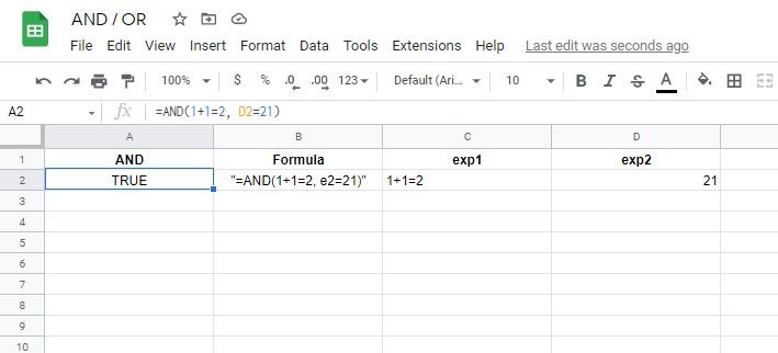
=AND(exp1, exp2)
In this formula, the first argument is needed, and the second one is optional.
- exp1 - This is the first expression to be input inside the formula. It can contain a cell address or a direct argument. The value should be something that can represent a logical value like TRUE or FALSE.
- exp 2 - This is an optional value. Once added, both values need to be either TRUE or FALSE for the AND function to return a result. You can add more expressions if you choose.
How to Use the AND Function
Here are the steps to follow to use the AND function in Sheets:
Click on the cell where you want to type in the function.
- Type in =AND( then write your first argument.
- Add a comma, and then write your second argument if needed.
- Close the function with a closing bracket and press Enter.
Examples of the AND Function
To help you understand the AND function better, here are a few examples of this formula in action.
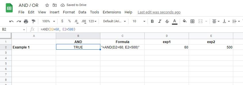
Example 1: Finding TRUE Values With the AND Function
In this scenario, we compare the values in two different cells to see if they match the ones provided in the formula. In this case, both arguments are TRUE, which means the value for AND is also TRUE.
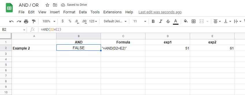
Example 2: Finding False Values With the AND Function
In this case, we deliberately made a situation where two inputs can not be equal. We get a FALSE output when adding this argument into the AND formula.
The Syntax for the OR Function
Here is the syntax for the OR function in Google Sheets:
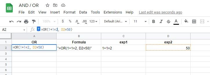
=OR(exp1, exp2)
Similar to the AND function, the first argument is needed, and the second one is optional.
- exp1 - This is the first expression to be input inside the formula, and it can contain a cell address or a direct argument. The value needs to be something that can represent a logical value like TRUE or FALSE.
- exp 2 - This is an optional value. Once added, both values need to be either TRUE or FALSE for the OR function to be true. Again, you can add more expressions if you need to.
How to Use the OR Function
Here are the steps to follow to use the OR function in Sheets:
- Click on the cell where you wish to execute the function.
- Type in =OR( and then write your first argument.
- Add a comma and write your second argument.
- Close the function with a closing bracket and press Enter.
Examples of the OR Function
In the demonstration, both of the arguments give the output as TRUE. Now, let's look at other examples to better understand the output in different circumstances.
Example 1: Finding TRUE Values With the OR Function
In this scenario, the first input will obviously give the wrong answer. However, the second argument will give a TRUE output that satisfies the OR function as it only needs one value to be true.
Example 2: Finding FALSE Values With the OR Function
In this case, we input the argument as the two values not being equal. However, both cells contain the same values, meaning the output returned is FALSE.
The Difference Between AND and OR Functions in Google Sheets
Both of these functions are a great way of ensuring your data is valid in Google Sheets. There are almost no differences between the AND and OR functions, except:
- The AND function requires all the arguments in the formula to return the value as TRUE to give a TRUE result.
- The OR function requires any one of the arguments to return a true value of TRUE to return a TRUE result.
Nesting AND With OR in Google Sheets
Let's look at a practical example of nesting AND/OR. Let's pretend we are a teacher of a safety course. The students need to have passed 2 tests or completed an extracurricular course to get a passing grade for the semester. The passing test mark is 5/10 and the extracurricular course is an ungraded pass upon completion. Here's how we could show that in a spreadsheet.
In the above example, we used the AND function as the first argument of the OR function. This is because the students needed to pass both tests. So the score in B2 and C2 must both be equal to or greater than 5 shown by the >= operator.
The second argument in the OR function is D2="Yes" which shows that students completed the extra training. If they meet either of the conditions, the formula will show a TRUE value. If neither of the conditions, a FALSE value will be returned.
Nested Functions With IF & AND/OR
To correctly understand nested IF functions with the AND and OR functions, we first need to properly understand the IF function itself. Here is the syntax for it:
=IF(exp, val_true, val_false)
Here are the arguments needed for the IF function:
- exp - This is a reference to a cell or a value checked to see if TRUE or FALSE.
- val_true - This is the value to display if the exp argument returns as TRUE.
- val_false - This is an optional argument displayed if the exp argument is FALSE.
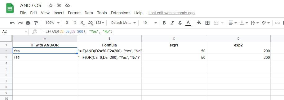
Now that we know how the IF and the AND/OR function work in Google Sheets, let's look at how we can use AND/OR in conjunction with the IF function to create a nested function.
The IF function will show any of the two specified values depending on the input of an argument. To understand, let's take a look at an example and some steps on how to do it.
- Click on the cell and start typing in =IF(
- Now, write =AND( or =OR( depending on your needs.
- Write your arguments in the AND/OR formula and add a closing bracket.
- Enter the values to return for TRUE and FALSE values, here we used “Yes” and “No”.
- Finally, add another closing bracket to close the IF function and press Enter.
When using the OR function with IF, only one of the arguments is needed to be true to satisfy the equation. Using the AND function with IF requires all of the arguments in the AND formula to be satisfied to return the TRUE value in the equation. You can nest IF Excel functions similarly when importing or exporting documents too.
Keep Mastering Google Sheets
The AND and the OR functions are some of the most simple functions in Google Sheets. But, you can use them to make important calculations as part of larger nested formulas. There's still plenty more to learn about Google Sheets. Keep practicing, and you'll be a pro in no time.

