Perhaps you need to add formatting to your spreadsheet on Google Sheets quickly but don't have a PC in view; you can use Google Sheets on your smartphone instead. Like the web version, the Google Sheets mobile app gives you an avenue to format your spreadsheet like a pro.

We'll show you how to format a Google Sheets spreadsheet using the Android app in this article.

How to Select Cells for Formatting in Google Sheets Mobile App

An appropriate cell, column, or row selection is essential for a sleek formatting experience in the Google Sheets mobile app. Here's how to select cells appropriately during formatting:

Tap the column label at the top to select an entire column. Tap a row number for a whole row, or touch a cell to select a single cell. Drag the blue highlight around the first cell to the last one to highlight specific cells.

Now let's dive right into formatting your Google Sheets spreadsheet.

Apply Color Fill Formatting to Specific Cells

This option allows you to fill specific cells with colors in your spreadsheet. To apply color formatting to cells:

1. Select the column, row, or cell.
2. Tap the A icon at the top of the spreadsheet to enter the formatting menu.
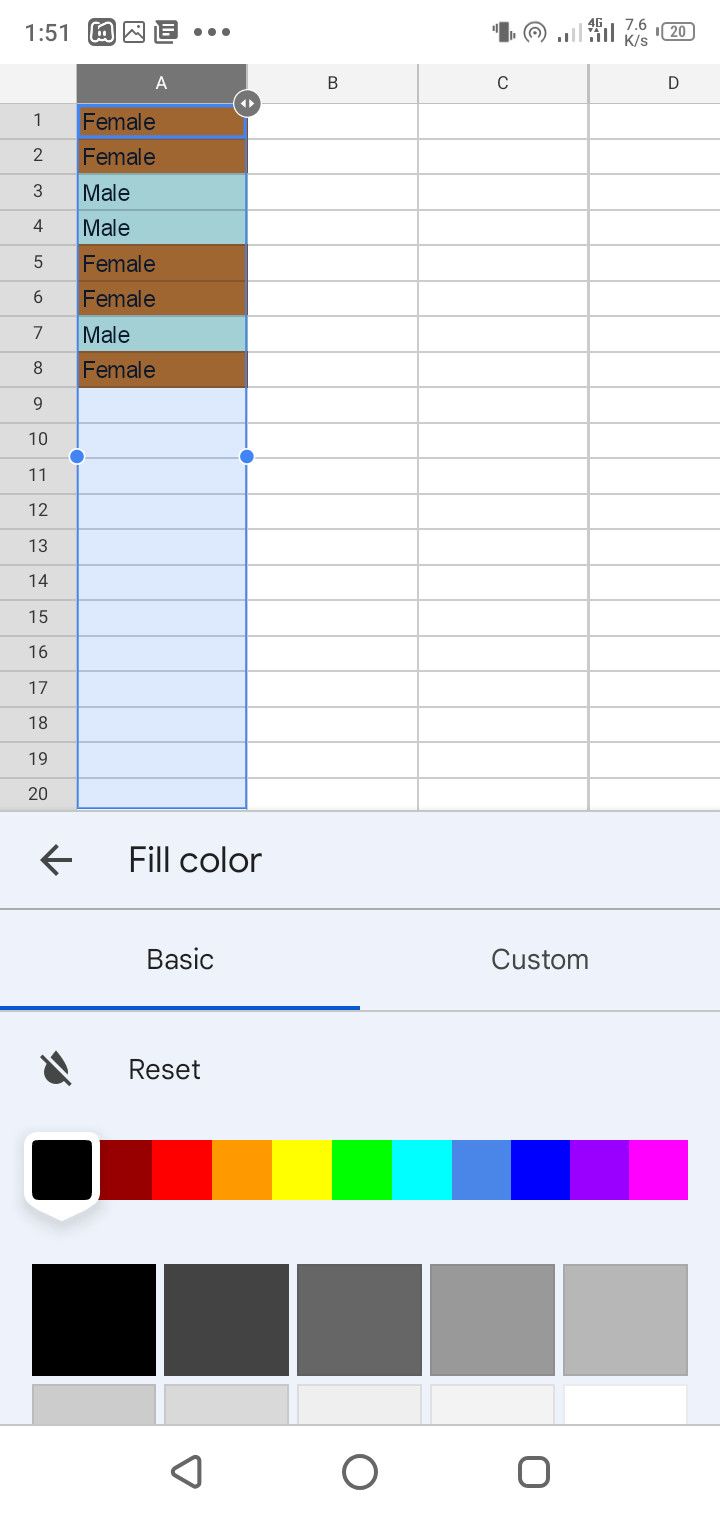
3. Go to the Cell section and tap Fill color.
4. Choose a color from the options to fill the selected fields.

For instance, to fill up a specific row, select that entire row and follow the above steps to fill the cells with your chosen color.

Format Borders in a Google Spreadsheet

You can also change the border style and color for selected columns, cells, or rows. To format the borders in a Google Sheets spreadsheet on mobile:

1. Select the cell, row, or column.
2. Go into the formatting menu by tapping the A icon at the top of the spreadsheet.
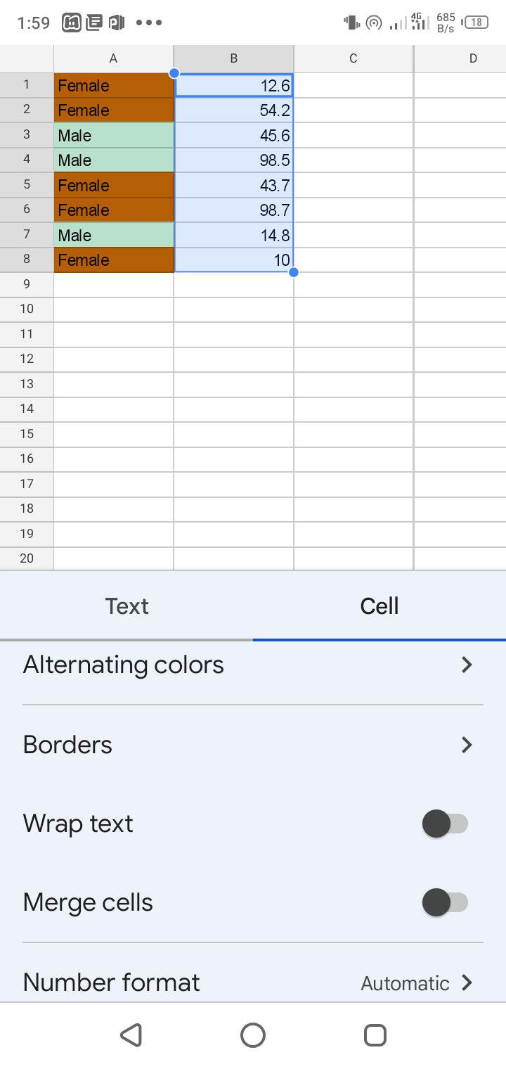
3. Select the Cell section and tap Borders.
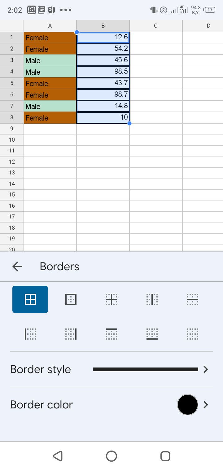
4. Next, choose a border type from the options.
5. Also, you can tap Border style and choose a line width to adjust the border thickness.
6. To apply color to selected borders: Tap Border color and pick from the color options.

Change Column Entry Format

You can specify the column, row, or cell input type in the Google Sheets mobile app:

1. Select the cell, row, or column you want.
2. Tap the A icon at the top to enter the formatting menu.
3. Go to the Cell section of the formatting menu.
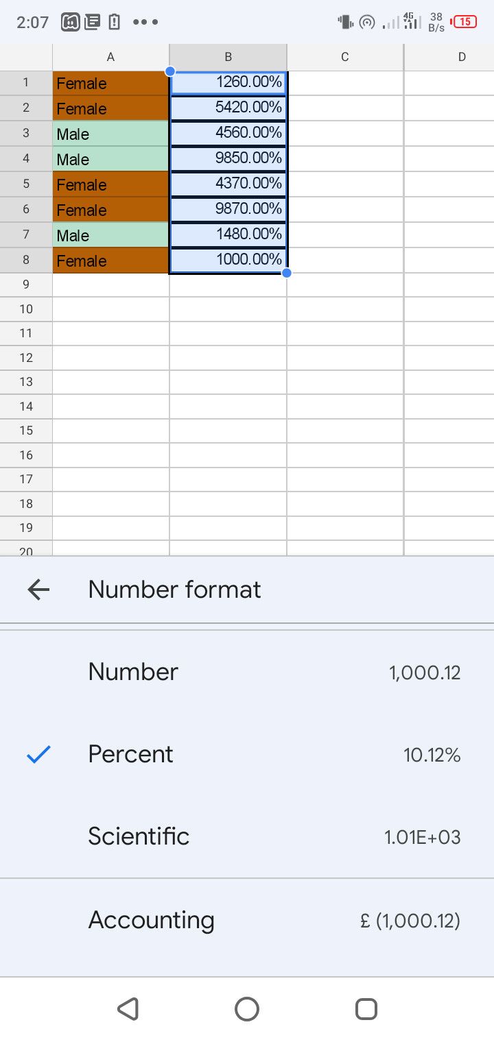
4. Select Number format. Then choose an appropriate format from the options.
5. For instance, you can use Plain text for non-numeric inputs or select Percent, Number, or any other applicable option for integer inputs.

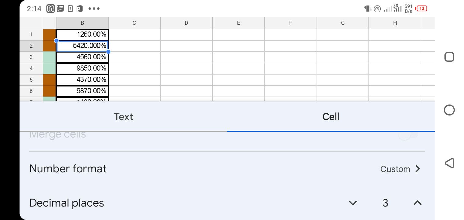
Format Number Into Decimal Places

This formatting option is only applicable to number entries. And it's straightforward:

1. Select the cells that'll use decimal places.
2. Tap A at the top of the spreadsheet.
3. Go to the Cell section.
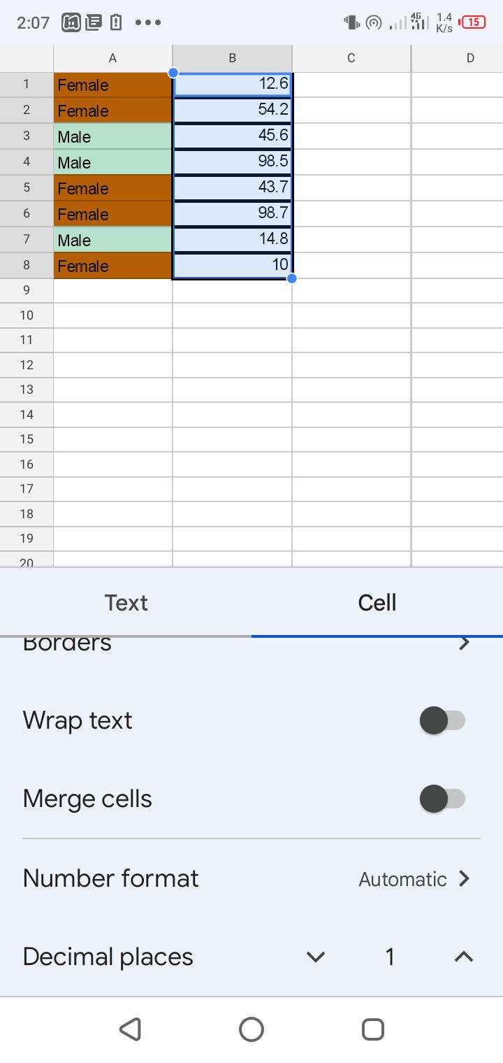
4. You'll see the Decimal places option at the tail end of that section.
5. Use the up and down pointers to the right to increase or decrease the number of decimal places.

Format Font Size and Font Type in Google Sheets Mobile App

Perhaps you want to use a specific font style or size for selected columns, rows, or cells:

1. Select the concerned cells and tap the A icon at the top to enter the formatting menu.
2. Go to the Text section to use either formatting option.
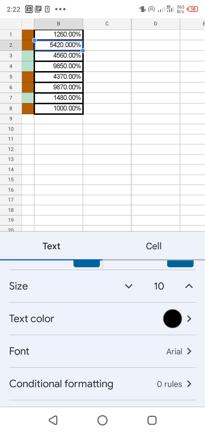
3. Tap the pointers to the right of the Size option to increase or decrease the font size of all entries in the selected cells.
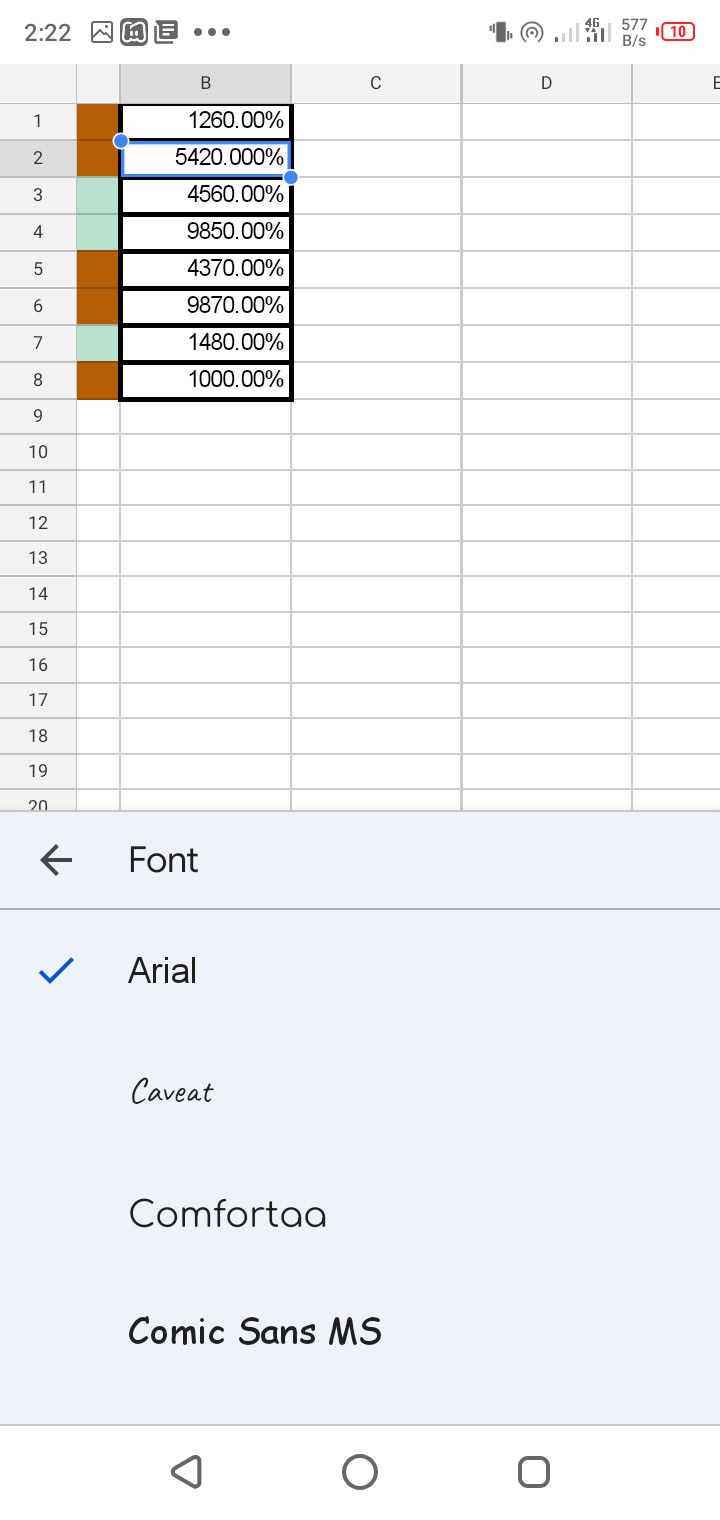
4. Also, select Font and pick from the font options that appear to change the text font for the chosen areas.

How to Rotate Text Entries in Google Sheets Mobile App

Sometimes you might need to tilt a cell entry for consistency or better presentation:

1. Tap the formatting icon (A) at the top of the spreadsheet.
2. Go to the Text section.
3. The tap Text rotation.
4. From here, you can choose to tilt or rotate the texts up or down or stack them vertically.

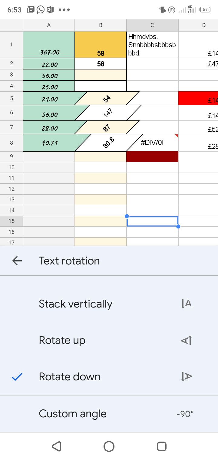
However, you can also use the custom option by tapping Custom angle, which allows you to specify an angle of rotation.

Note: You can only use angles between -90 and 90 degrees when using the custom orientation. For instance, -95 degrees will not work since it's less than -90 degrees. Also, 95 degrees will not work since it's higher than 90 degrees.

How to Format Text Color

This formatting simply allows you to change the text color of your entries in selected cells:

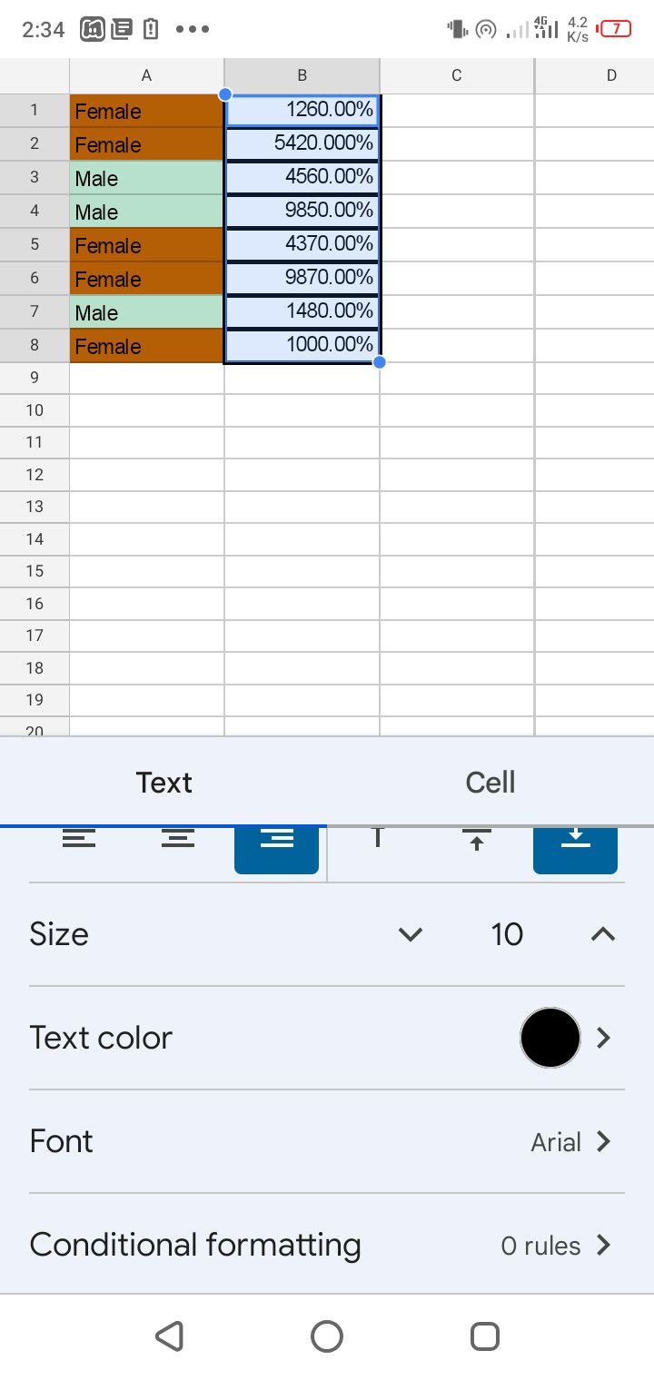
1. Select a column, row, or cell and tap the formatting icon (A) at the top.
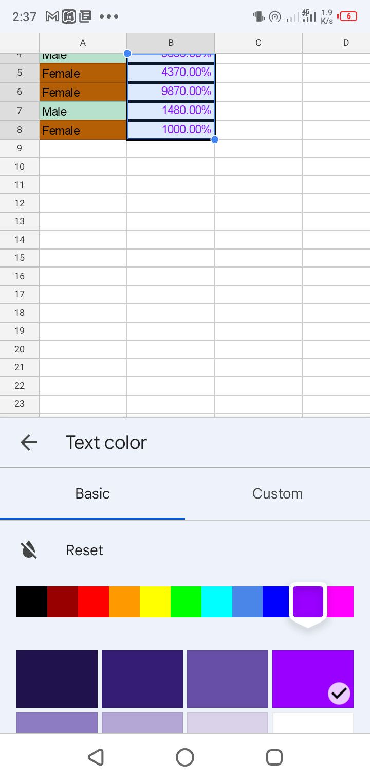
2. Select Text color from the Text section.
3. Next, pick your chosen color from the options.

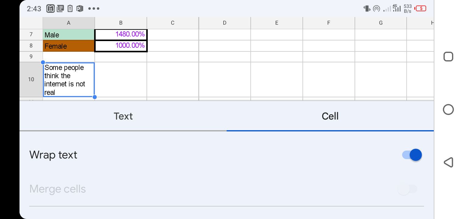
Wrap Text to Fit a Cell

Like its desktop version, the Google Sheets mobile version also features a text wrapper that allows a text to fit into a cell, regardless of its length:

1. Choose the column, cell, or row you want to wrap its texts.
2. Tap the A icon at the top to open the formatting menu.
3. Go to the Cell section.
4. Next, toggle on the switch to the right of Wrap text.

Strikethrough, Bold, Italicize, Highlight, and Align Texts

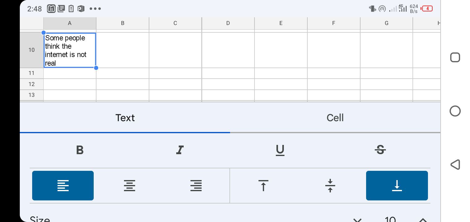
To start with any of these, select the area in your spreadsheet where you want to apply it. When you go to the Text section of the formatting menu, you'll see these formatting icons at the top of that section.

Select the B icon to bold the texts in a selected column, row, or cell. Tap I to italicize an entry, or tap the highlighted U to highlight a text. Next to this is the strikethrough icon. This gives a single stroke across a text.

Toggle between the vertically arranged alignment bars to switch between left, right, or middle text alignment. Immediately next to these alignment bars are two arrows for vertical alignment. Toggle between the double-facing and single arrows to use these vertical alignment options.

How to Use Conditional Formatting in Google Sheets Mobile App

Conditional formatting lets you organize your spreadsheet how you like, as it provides several custom formatting options and lets you use Google Sheets like a pro. Unfortunately, the iOS version of Google Sheets doesn't feature conditional formatting. But the Android version does.

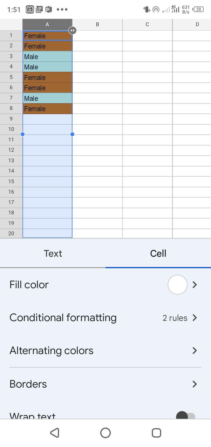
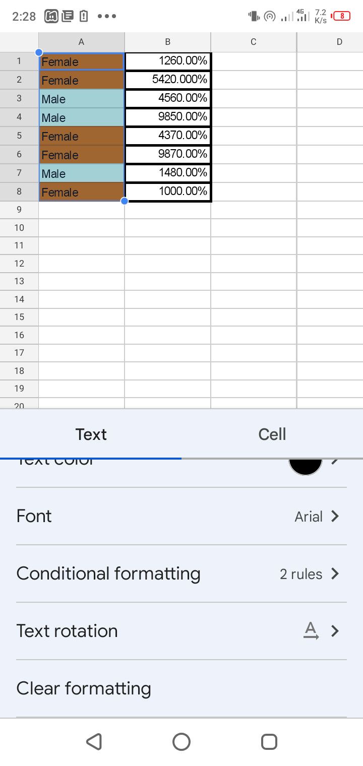
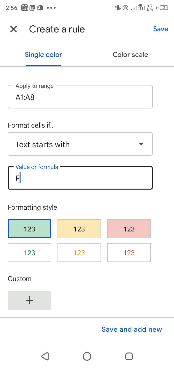
For instance, to differentiate between male and female entries using different colors, you can use the Starts with conditional formatting system:

1. First, highlight the cells you want to format in a column by dragging the blue highlight around the first cell to the last one.
2. Tap the A icon at the top to open the formatting menu. Then tap Text or Cell.
3. Select Conditional formatting.
4. Next, tap the dropdown under Format cells if.
5. Select Text starts with. Then type the value F in the Value or formula field to represent the female entries.
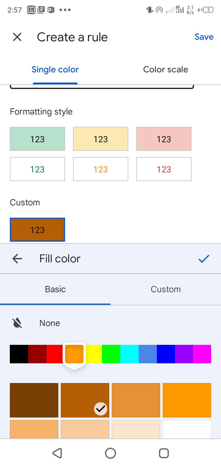
6. Choose a cell fill and text color under Formatting styles. The first set of colors is for filling the cells, while the second one represents text colors. But you can use custom color options instead.
7. To use custom color options, tap the + icon right under Custom. Tap Text color or Fill color to apply custom color to all the female entries.
8. Tap the checkmark at the top-right of that submenu to apply changes. Then tap Save and add new at the bottom-right.
9. Repeat the same process for the male entries. But this time, you'll type M in the Value or formula field to signify male entries.
10. Ensure to use a different color for each entry. You can repeat this process for as many entry categories as you have.
11. Finally, tap the checkmark at the top-left to apply the formatting.

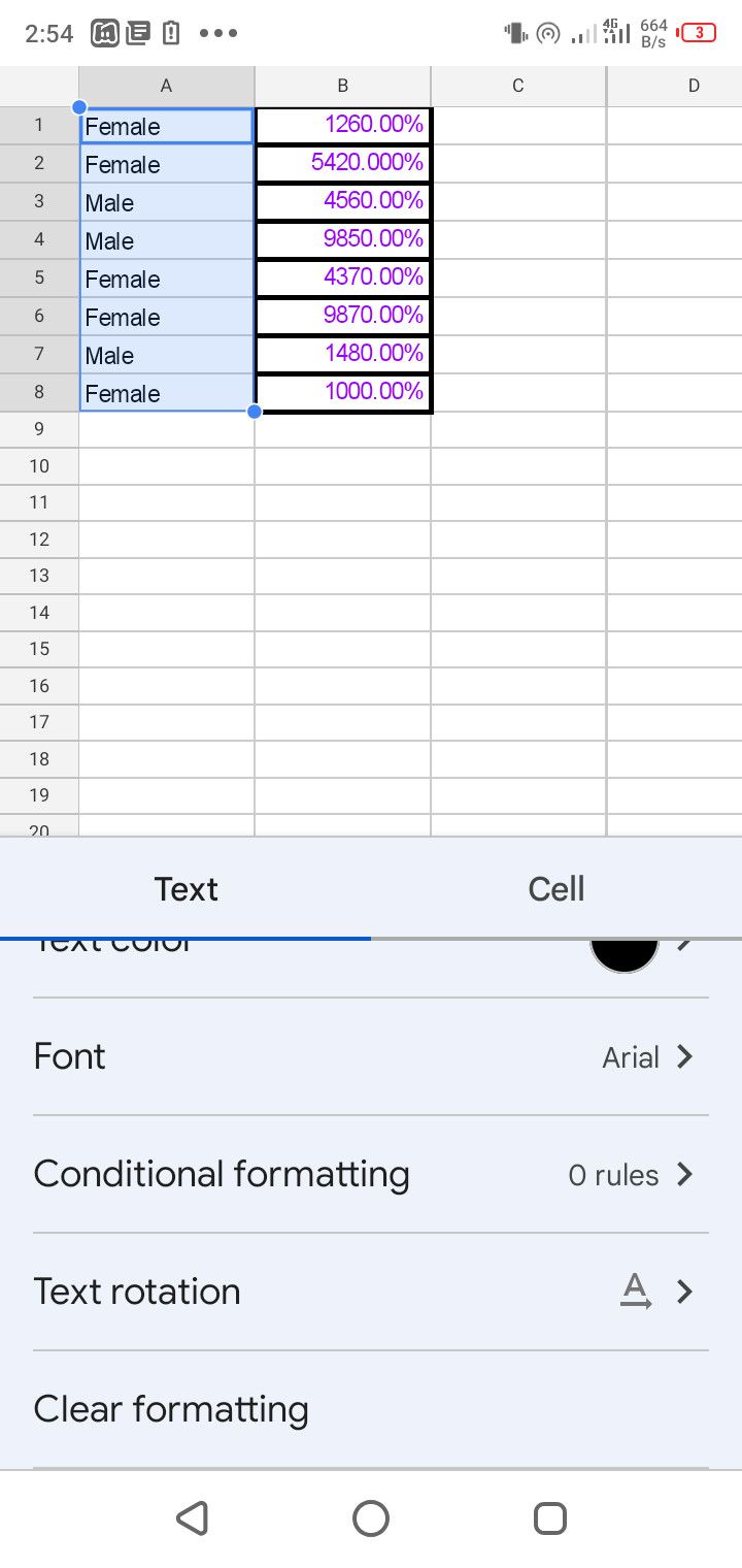
Keep in mind that Conditional formatting supports many conditions. So it applies to number entries, too. There's even a custom option if you prefer to write your Google Sheets formulas from scratch.

Format Your Google Spreadsheet Like a Pro on the Mobile App

The Google Sheets mobile app can be a handy tool to use anywhere if you're not with a computer. It lets you format your spreadsheet as you would in the web version. You might not need to use the web version anymore once you have a solid grasp of using the mobile version.

And thankfully, your work syncs across all devices. So you can jump right in from anywhere. You might also want to see some tips for formatting your Google Sheets like a pro.