Key Takeaways

• Excel’s VLOOKUP may seem tricky, but with practice, you'll master it easily.
• The formula lets you search for a value in a table and returns a corresponding one.
• VLOOKUP helps with data analysis, GPA calculation, and comparing columns.

VLOOKUP might not be as intuitive as other functions, but it’s a powerful tool worth learning. Take a look at some examples and learn how to use VLOOKUP for your own Excel projects.

What Is VLOOKUP in Excel?

Excel's VLOOKUP function is similar to a telephone book. You provide it with a value to look up (like someone’s name), and it returns your chosen value (like their number).

VLOOKUP might seem daunting at first, but with a few examples and experiments, you'll soon be using it without breaking a sweat.

The syntax for VLOOKUP is:

        =VLOOKUP(lookup_value, table_array, col_index_num[, exact])
    

This spreadsheet contains sample data to show how VLOOKUP applies to a set of rows and columns:

In this example, the VLOOKUP formula is:

        =VLOOKUP(I3, A2:E26, 2)
    

Let's see what each of these parameters means:

• lookup_value is the value that you want to look up in the table. In this example, it's the value in I3, which is 4.
• table_array is the range that contains the table. In the example, this is A2:E26.
• col_index_no is the column number of the returned desired value. The color is in the second column of table_array, so this is 2.
• exact is an optional parameter determining whether the lookup match should be exact (FALSE) or approximate (TRUE, the default).

You can use VLOOKUP to display the returned value or combine it with other functions to use the returned value in further calculations.

The V in VLOOKUP stands for vertical, meaning that it searches a column of data. VLOOKUP only returns data from columns to the right of the lookup value. Despite being limited to the vertical orientation, VLOOKUP is an essential tool that makes other Excel tasks easier. VLOOKUP can come in handy when you're calculating your GPA or even comparing two columns.

VLOOKUP searches the first column of table_array for lookup_value. If you want to search a different column, you can shift the table reference, but remember that the return value can only be to the right of the search column. You may choose to restructure your table to meet this requirement.

How to Do a VLOOKUP in Excel

Now that you know how Excel's VLOOKUP works, using it is just a matter of choosing the right arguments. If you find typing the arguments difficult, you can start the formula by typing in an equal sign (=) followed by VLOOKUP. Then click the cells to add them as arguments in the formula.

Let's practice on the sample spreadsheet above. Assume you have a spreadsheet containing the following columns: Name of products, Reviews, and Price. You then want Excel to return the number of reviews for a particular product, Pizza in this example.

You can easily achieve this with the VLOOKUP function. Just remember what each argument will be. In this example, since we want to look up information about the value in cell E6, E6 is the lookup_value. The table_array is the range containing the table, which is A2:C9. You should only include the data itself, without the headers in the first row.

Finally, the col_index_no is the column in the table where the reviews are, which is the second column. With these out of the way, let's get to writing that formula.

1. Select a cell where you want to display the results. We'll go with F6 in this example.
2. In the formula bar, type =VLOOKUP(.

   

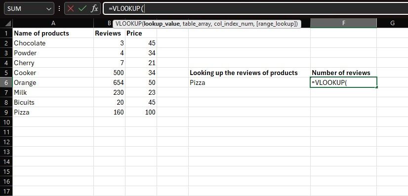
3. Highlight the cell containing the lookup value. That is E6 in this example, which contains Pizza.
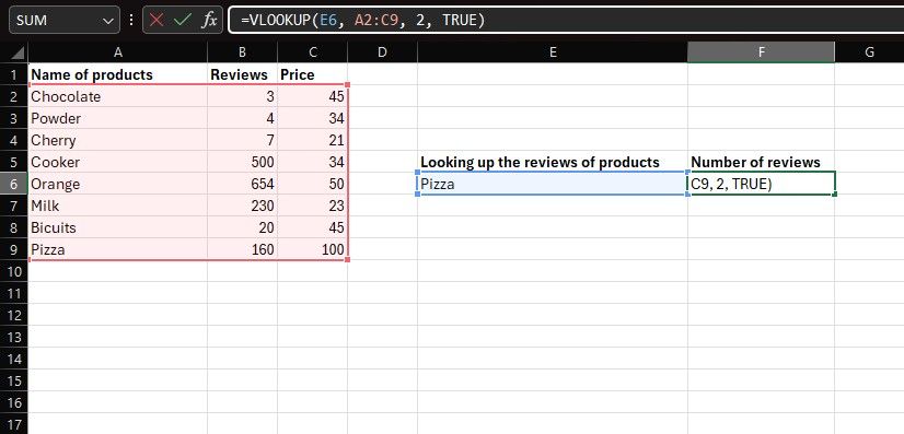
4. Type a comma (,) and a space, and then highlight the table array. That is A2:C9 in this example.
5. Next, type in the column number of the desired value. The reviews are in the second column, so that's 2 for this example.
6. For the last argument, type FALSE if you want an exact match of the item you entered. Otherwise, type TRUE to see the closest match for it.

   

7. End the formula with a closing parenthesis. Remember to put a comma between the arguments. Your final formula should look like below:

           =VLOOKUP(E6,A2:C9,2,FALSE)
       

8. Hit Enter to get your result.

   

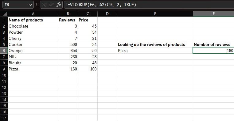
Excel will now return the reviews for Pizza in cell F6.

How to Do a VLOOKUP for Multiple Items in Excel

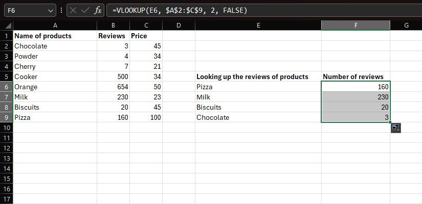
You can also look up multiple values in a column with VLOOKUP. This can come in handy when you need to perform operations like plotting Excel graphs or charts on the resulting data. You can do this by writing the VLOOKUP formula for the first item and then auto-filling the rest.

The trick is to use absolute cell references so they don't change during autofill. Let's see how you can do this:

1. Select the cell next to the first item. That's F6 in this example.
2. Type the VLOOKUP formula for the first item.
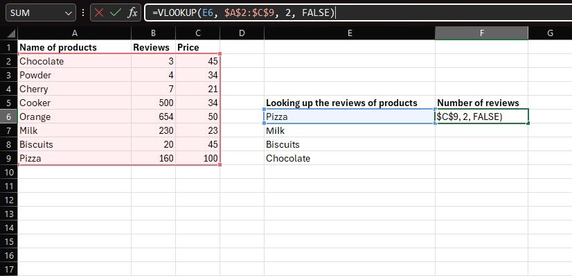
3. Move your cursor to the table array argument in the formula and press F4 on your keyboard to make it an absolute reference.

   

4. Your final formula should look like below:

           =VLOOKUP(E6,$A$2:$C$9,2,FALSE)
       

5. Press Enter to get the results.
6. Once the result appears, drag the results cell down to fill the formula in for all the other items.

   

If you leave the final argument blank or type TRUE, VLOOKUP will accept approximate matches. However, the approximate match can be too lenient, particularly if your list is not sorted. As a general rule, you should set the final argument to FALSE when searching for unique values, such as the ones in this example.

How to Connect Excel Sheets With VLOOKUP

You can also draw information from one Excel sheet to another using VLOOKUP. This is particularly useful if you want to leave the original table unaffected, like when you've imported the data from a website to Excel.

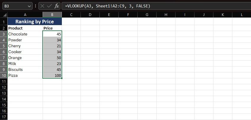
Imagine that you've got a second spreadsheet where you want to sort the products from the previous example based on their price. You can get the price for these products from the parent spreadsheet with VLOOKUP. The difference here is that you'll have to go to the parent sheet to select the table array. Here's how:

1. Select the cell where you want to display the price of the first item. That's B3 in this example.
2. Type =VLOOKUP( in the formula bar to start the formula.

   

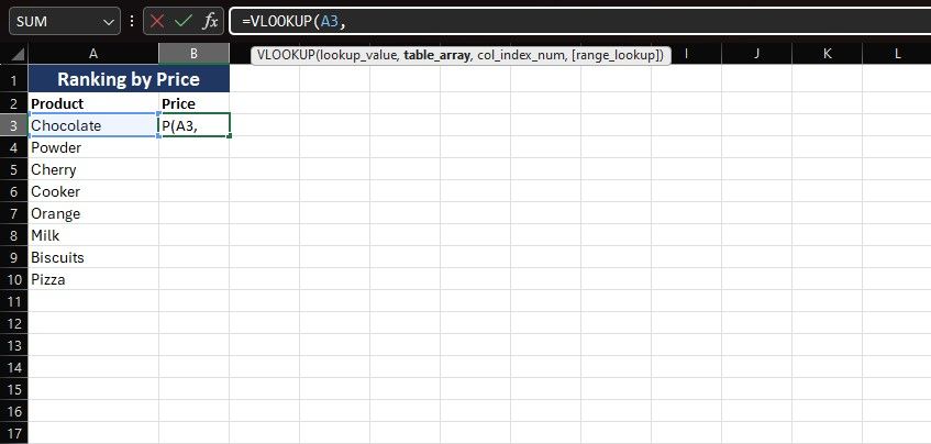
3. Click the cell containing the first item's name to append it as the look-up value. That's A3 (Chocolate) in this example.
4. Like before, type a comma (,) and a space to move to the next argument.
5. Navigate to the parent sheet and select the table array.

   

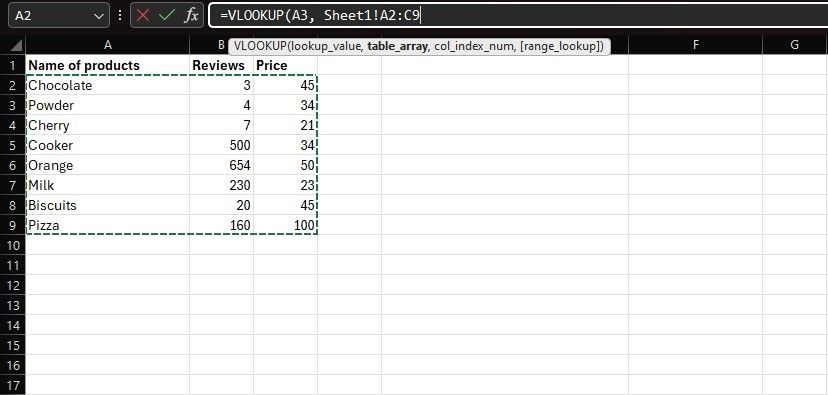
6. Hit F4 to make the reference absolute. This makes the formula applicable to the rest of the items.
7. While still on the parent sheet, look at the formula bar and type the column number for the price column. That's 3 in this example.
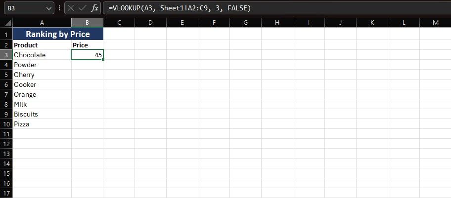
8. Type FALSE since you want an exact match of each product in this case.

   

9. Close the parenthesis and hit Enter. The final formula should look like below:

           =VLOOKUP(A3, Sheet1!$A$2:$C$9, 3, FALSE)
       

10. Drag down the result for the first product to see results for the other products in the subset sheet.

    

You can now sort your Excel data without it affecting the original table. Typos are one of the common causes of VLOOKUP errors in Excel, so make sure to avoid them in the new list.

VLOOKUP is a great way to query data faster in Microsoft Excel. Although VLOOKUP only queries within a column and has a few more limitations, Excel has other functions that can do more powerful lookups.

Excel's XLOOKUP function is similar to VLOOKUP but can look both vertically and horizontally in a spreadsheet. Most of Excel's lookup features follow the same process, with only a few differences. Using any of them for any specific lookup purpose is a smart way to get a hold of your Excel queries.