When you work with large data sets in a spreadsheet, you will often have to traverse around downwards or to the right. But, when comparing or analyzing data, you might want to keep some of the data permanently in your view.

This can make it much easier to know what each row and column represents by keeping the headers in place or making important data points visible. Thankfully, Google Sheets allows you to freeze rows and columns. Read on to learn what this feature does, why you’d use it, and the steps involved in Google Sheets for web and mobile.

Why Freeze Rows and Columns in Google Sheets?

The freezing feature in Sheets allows you to pin your desired rows or columns in your spreadsheet. That way, you can always have them in view when you scroll through the spreadsheet.

This feature can be a lifesaver if you work with massive spreadsheets that span several pages. Not using this feature means that the header cells will move when you scroll through the spreadsheet, making it confusing to know which cell is under what name.

You’d want to freeze rows and columns in Sheets for the same reasons you’d like to freeze panes in Excel. Here are some of the situations where freezing a row or column might be beneficial to you:

• To keep headers locked in their place to identify the key rows and columns of the data.
• To compare important data points with other data in the spreadsheet.
• Keep a reminder of some of the key data in the spreadsheet.

Most of the time, you will only want to freeze the first row or column in the spreadsheet. However, you can freeze multiple rows or columns if you need to, as long as they are side by side. There are a few things you should know about this formatting feature in Google Sheets. These are:

• You can’t freeze standalone rows or columns that are in the middle of the spreadsheet. You can only choose these if they are next to the first row or column. You may have to sort your columns in Google Sheets first.
• You can’t simultaneously freeze the rows and the columns. You will have to freeze the rows or columns one after the other.

How to Freeze Rows or Columns in Google Sheets

You can freeze the rows and columns in Google Sheets in multiple ways. Here’s how to do it.

Using the Mouse

This is one of the easiest ways to freeze rows or columns in your spreadsheet. All you have to do is click and drag a specific part in the spreadsheet.

Here are the steps you need to follow to do this:

1. In your spreadsheet, take your mouse cursor to the top-left part of the spreadsheet. You will see an empty box beside the A and the 1 used to represent the rows and columns.
2. You will see two thick gray lines (bars), one towards the right side of the box and the other one at the bottom. Hover your cursor over these lines. The cursor will change to a palm icon.
3. Left-click and hold the appropriate bar and drag it to the right or downwards, depending on if you want to freeze rows or columns.

For example, if you drag the horizontal bar down below row 1, row one will be frozen. If you drag it below row 2, rows 1 and 2 will be frozen, etc.

The same goes for columns. If you drag the gray bar to the right of column A, it will freeze column A. If the gray line is to the right of column B, columns A and B will both be frozen, etc. In the screenshot below, you can see that rows 1-3 are frozen and so are rows A-C.

Using Options Menu

Although using the mouse is a much easier way to freeze rows and columns in Google Sheets, there is another way to do this. Here are the steps you need to follow to use the options menu to freeze rows in Google Sheets:

1. Open the spreadsheet on the web version of Google Sheets.
2. Click on View in the top main bar of the spreadsheet.
3. Now, click on Freeze in the dropdown menu that shows up.
4. Here, you can choose whether you want to choose rows or columns to freeze and the number of them. Simply click on the desired option to freeze them.

The dropdown menu only shows up to 2 rows and columns. If you want to freeze more than 2 rows and columns, click on the cell up to which you want to freeze first. Then click on View and then on Freeze. There, you can choose the Up to row X or Up to column X option from the menu.

This will lock the first X number of rows or columns, meaning they will stay visible when you scroll through the spreadsheet. You can't freeze the rows and columns at once, so you have to do them one by one.

For Android and iOS

Here are the steps to follow in order to freeze rows or columns on mobile:

1. Open Google Sheets on your mobile.
2. There, open the desired spreadsheet.
3. Tap on the spreadsheet tab name (eg Sheet1) to open the options that allow you to make tweaks to your spreadsheet.

   

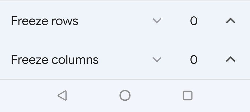
4. A smaller window will show up from the bottom side of the screen. Scroll down and use the up and down arrows to increase or decrease the number of rows and columns you want to freeze.

   

5. Finally, click out of the window to finalize the changes.

How to Unfreeze Rows and Columns in Google Sheets

Now that we know how to freeze the cells, let's look at how you can unfreeze the rows and columns in Google Sheets. This method is pretty much the exact opposite of the ones we used to freeze the cells. You can drag the thin gray lines back to their original position to unfreeze the rows and columns.

Alternatively, you can use the freeze option in the view menu. For example, let’s say you wanted to remove the freeze from both the rows and columns on your spreadsheet. Here are the steps you need to follow to do this:

1. Click on the View button in the top main menu.
2. Now, click on Freeze in the dropdown menu that shows up.
3. Click on the No Row option.
4. Now, click the View option again.
5. Click again on the Freeze in the dropdown menu that shows up.
6. Click on No Column.

Wrapping Up Freezing Rows and Columns

The above guide showed you how to simply freeze and unfreeze rows and columns in Google Sheets. This fundamental skill will make it much easier for you to work within your spreadsheets. All of your basic spreadsheet navigation should be more straightforward from now on.