When you owe a debt to a bank or lending institution, they usually give you a statement to see how much you've paid. However, that's about it. They can compute how much you have left to pay and for how long, but you'll have to get customer service to ask for it.
Some institutions also offer online calculators—however, these usually only work with fixed interest rates. If your loan uses variable interest rates, you'll have to figure it out yourself. Fortunately, you can create an Excel amortization table with changing interest rates. Here's how you can build it.
Building the Variable Rate Loan Amortization Table
Before building the table, you must have the following information on hand:
- The total loan amount
- The loan term (number of years to pay)
- The number of payments per term (number of payment periods in a year)
You also need to be familiar with the following formula:
-PMT(RATE,NPER,PV)
RATE refers to the annual interest rate applicable for that payment, NPER refers to the number of payments remaining, and PV refers to the remaining loan balance before the payment for the said period.
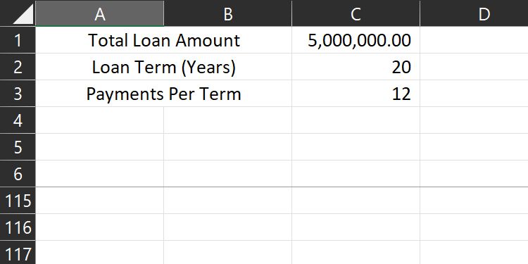
Once you have that information, input them into your Excel file. For this example, we will use a 20-year, $5,000,000 mortgage paid monthly.
After adding your initial data, you can start creating the amortization table.
Creating the Columns for Your Amortization Table
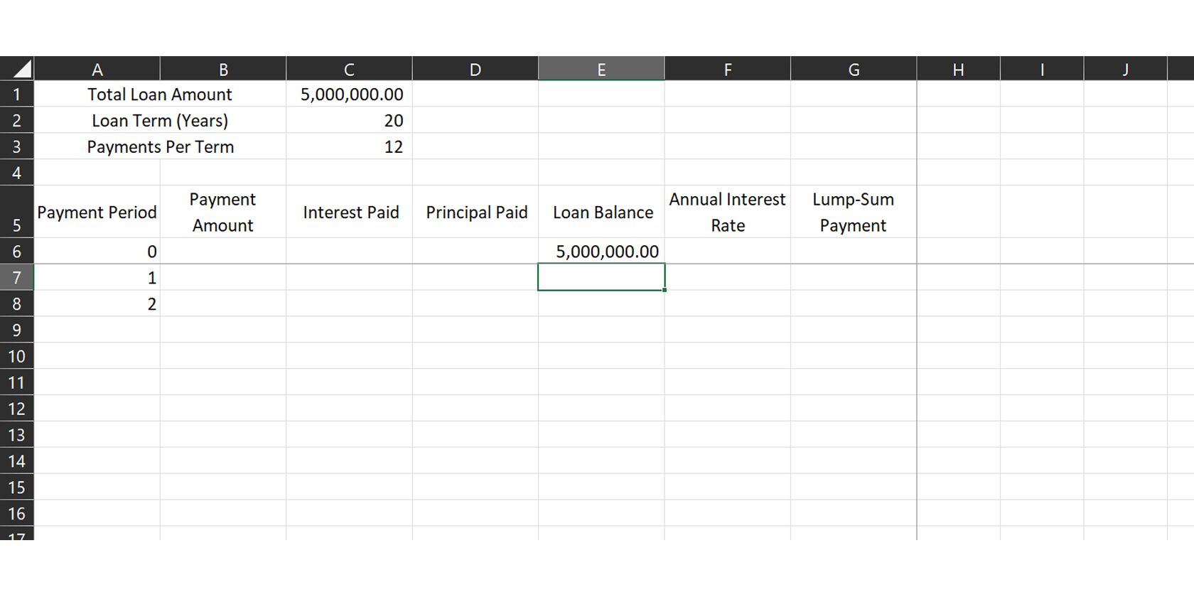
You need to create the following columns for your table:
- Payment Period: shows the payment period.
- Payment Amount: the total amount that must be paid for the period.
- Interest Paid: payment amount that goes to interest.
- Principal Paid: payment amount for reducing the original balance.
- Loan Balance: total loan amount remaining for payment.
- Annual Interest Rate: the annual interest rate for that payment period.
- Lump-Sum Payment: records advanced payments, if any.
Filling Out Fixed Data
Once you've created your columns, it's time to fill out pre-determined information. Under the Payment Period column, write 0 for your initial data, 1 in the next row to show the first payment period, and 2 in the row after that. After doing so, select all three cells.
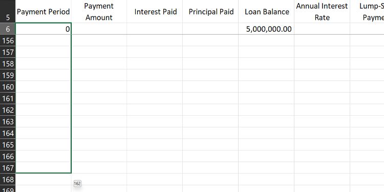
Once you've selected them, place your cursor on the green box at the lower-right corner of the selection box until it turns into a thin, black cross. From there, click on the box and then drag it downwards.
You should see a small box appear to the right of your cursor. This number indicates the last number that Excel will fill out—release the mouse button when you hit the total number of payment periods for your loan (240 in our example).
Under Loan Balance, link the total loan amount in Period 0 to the original Total Loan Amount. For our example, use the formula =C1. Leave the rest of the rows blank.
Under Annual Interest Rate, input the interest rate for the said payment period. If you have a 5/1 ARM (adjustable-rate mortgage), the first five years of your loan have a fixed rate. Then it will adjust annually, based on the market, after that period.
For this example, we'll use a 3.57% interest rate for the first five years and then use varying rates based on historical rates.
Adding the Formulas
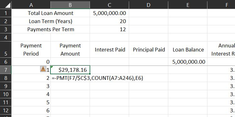
Once you've placed your placeholder interest rates, it's time to determine your first payment amount. Input the payment formula mentioned below in the Payment Period 1 row under the Payment Amount column.
=-PMT(RATE,NPER,PV)
Under RATE, choose the cell that lists the current annual interest rate (cell F6 in our example) and then divide it by the number of payments per period. Add the $ sign before the column and row indicator (cell $C$3 in our example) to ensure it doesn't change when you apply the formula to other cells later.
For NPER, type COUNT(. Afterward, select the first Period cell, press shift on your keyboard, then select the last Period cell (the current cell). Again, don't forget to add the $ sign before the column and row number in the formula that indicates the last cell ($A$245 in our example) to ensure it doesn't change later.
To input PV, select the cell containing the total loan amount in Period 0 (cell E6 in our example). Also, note that the PMT formula has a negative sign before it, so you get a positive value in your table. If you don't add this, you'll get a negative value.
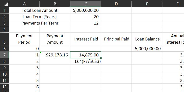
Under the Interest Paid column, compute the amount that goes to the interest in your monthly payment. Use the following formula:
=Balance Remaining*(Annual Interest Rate/Payments Per Period)
For our example, this is how the formula would look like:
=E6*(F7/$C$3)
Where E6 is the remaining balance you must pay, F7 is the current applicable Annual Interest Rate, and $C$3 is the number of payments you make per term.
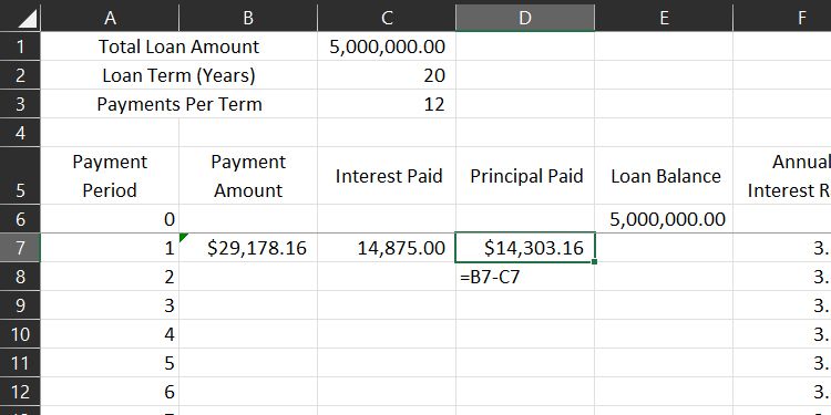
Once you've determined the amount of Interest Paid, subtract that from the Payment Amount to get the Principal Paid.
In our example, the formula is:
=B7-C7
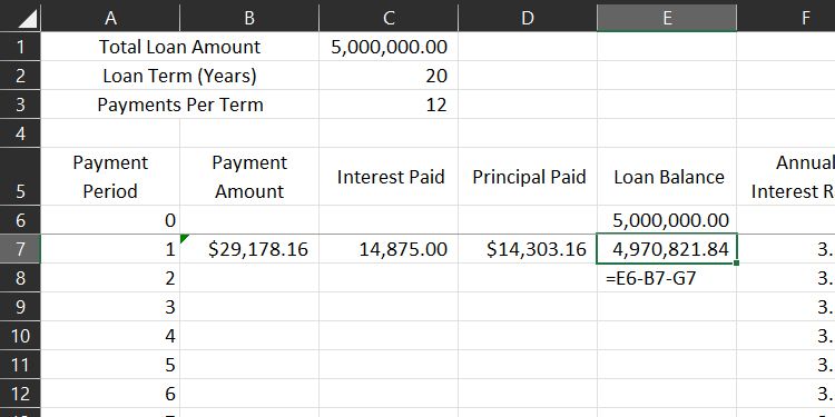
You can get the Loan Balance from there by subtracting the current Payment Amount and Lump-Sum Payment from the Loan Balance from the last period (Period 0).
This is what the formula looks like in our example:
=E6-B7-G7
Once you've added all the formulas, you should get all your first month's data ready.
Populating the Rest of Your Amortization Table
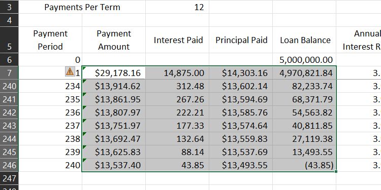
With all the initial formulas ready, you can now populate the rest of the table by just dragging and dropping. First, select the cells with a formula (Payment Amount, Interest Paid, Principal Paid, and Loan Balance under Period 1).
Then, place your cursor on the green box at the lower-right corner of the selection box until it turns into a thin, black cross. From there, click on the box and then drag it downwards to the last Payment Period. Once you reach the last row, release your mouse button, and Excel will fill out the rest of the cells for you.
Alternatively, you can Copy the cells with the formulas, then select all Payment Period rows under them. From there, select Paste or press Ctrl + V and Excel will automatically populate your table with the correct values.
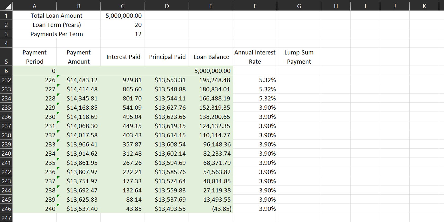
To avoid accidentally changing formulas, select all cells with a formula (cell A6 to cell E246) and then fill it in with any color. You can also use conditional formatting to change the color of your cells once your loan balance is fully paid off.
Experimenting With Your Data
Now that you've completed your initial table, you can freely change the Total Loan Amount to see its effect on your total loan. You can also change the Annual Interest Rate per Payment Period, allowing you to input actual data once your bank sends the effective rate of your loan. And if you have a little extra, you can make advance payments under Lump-Sum Payment.
Any change you make is accounted for by your formula, allowing you to get accurate results no matter what data you input, as long as it's valid. If you have a fixed-rate loan but want to experiment with the loan's duration, term, or monthly payments, check out how to create a fixed-rate amortization schedule in Excel.
Knowing Can Help You Plan Financially
With the variable-rate amortization schedule, you can plan your loan and payments. That way, you can prepare yourself, even if the interest rate changes. And with the lump-sum column, you can even see how small advanced payments can go a long way in helping you pay off your loan.


