You might know how to create a drop-down menu in Excel, but you might not know how to create multiple dependent drop-down menus.
There are various approaches to creating multiple drop-down menus, with some being easy to execute and others being difficult. This article explains how to do this relatively quickly with a single offset formula.
Example for Creating Multiple Dependent Drop-Down Lists
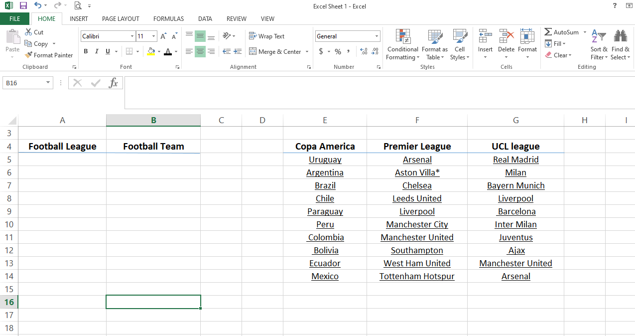
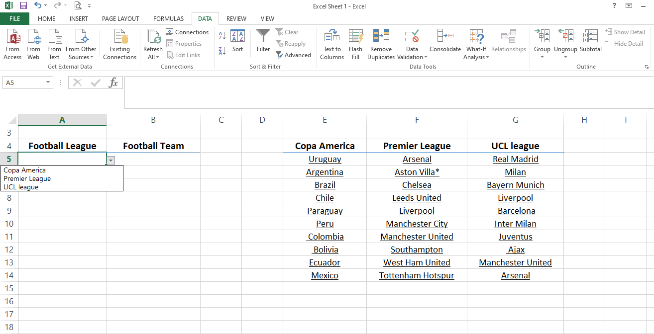
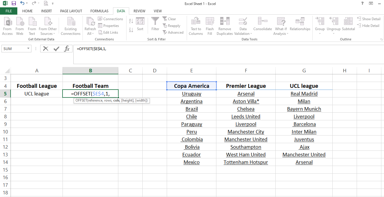
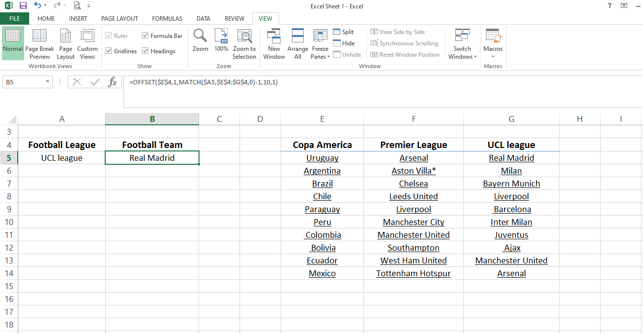
Let's take a look at the below data for which you intend to create a dependent drop-down list using the offset formula.
Here you can see three different leagues, each with its list of teams. In order to simplify the concept, each league can only have a small number of teams instead of featuring a full list.
On the left-hand side, you have two choices to select a league and its corresponding team. Your team selection will depend on what league you choose, as choice two is dependent on the first choice.
Our goal is to create a simple drop-down menu for league names and a dependent drop-down menu for each league's list.
Creating Simple Drop-Down Menu for Football Leagues
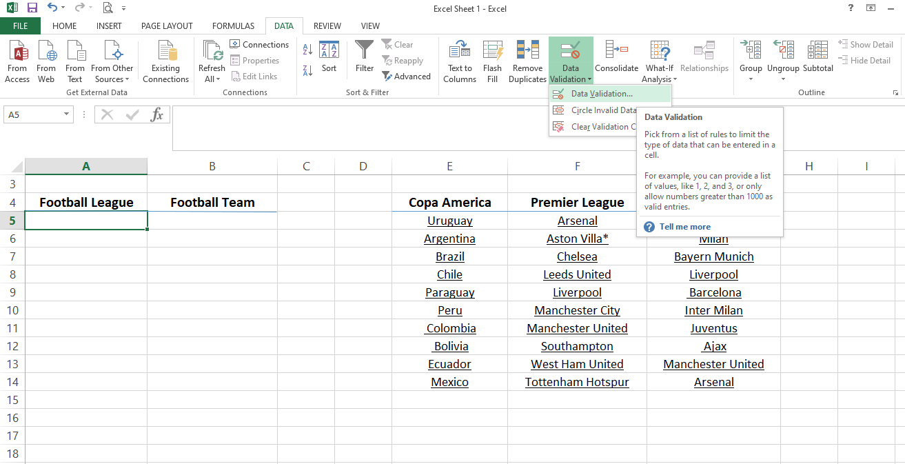
1. Go to the Data tab and click on Data Validation.
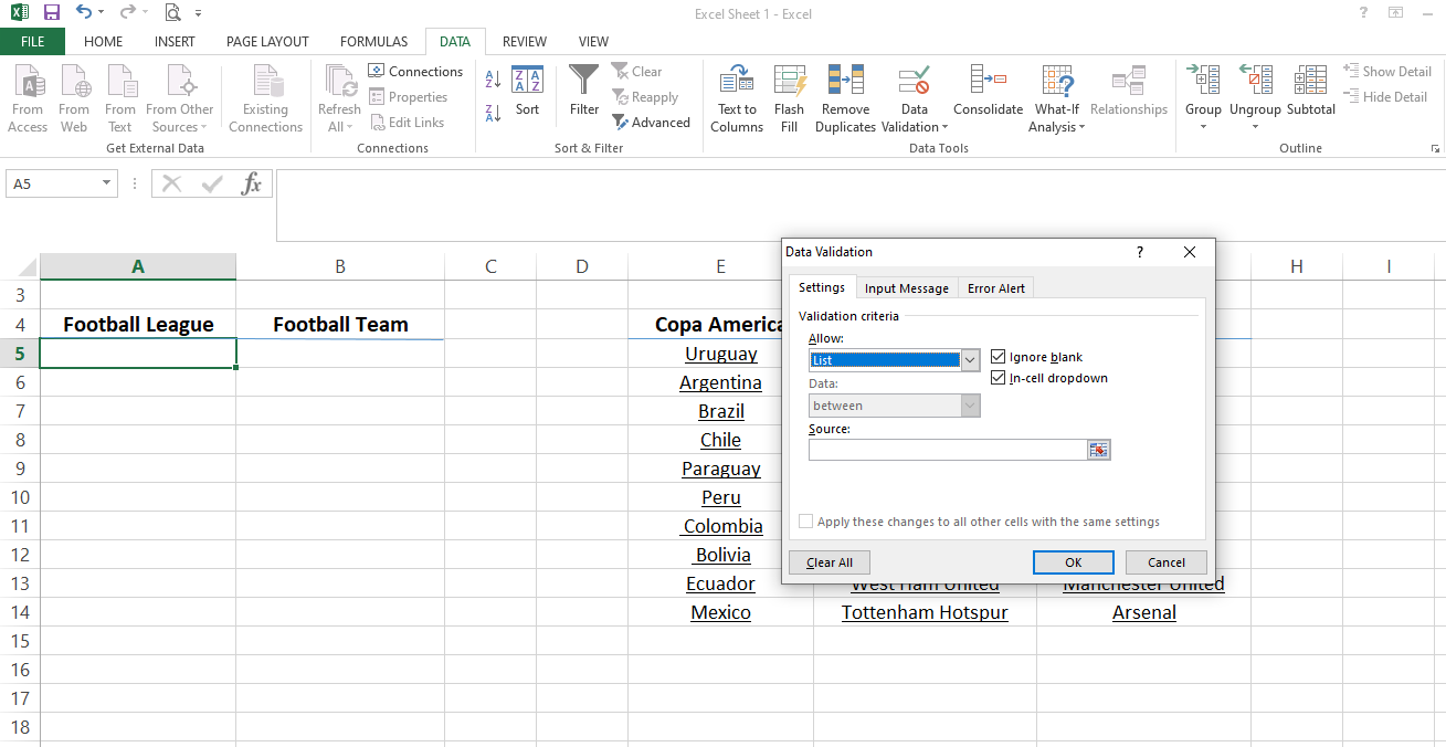
2. Select the List in Allow option in validation criteria.
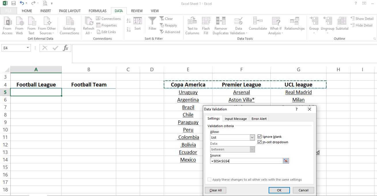
3. Select cells E4 to G4 as the source.
4. Click OK to apply the changes.
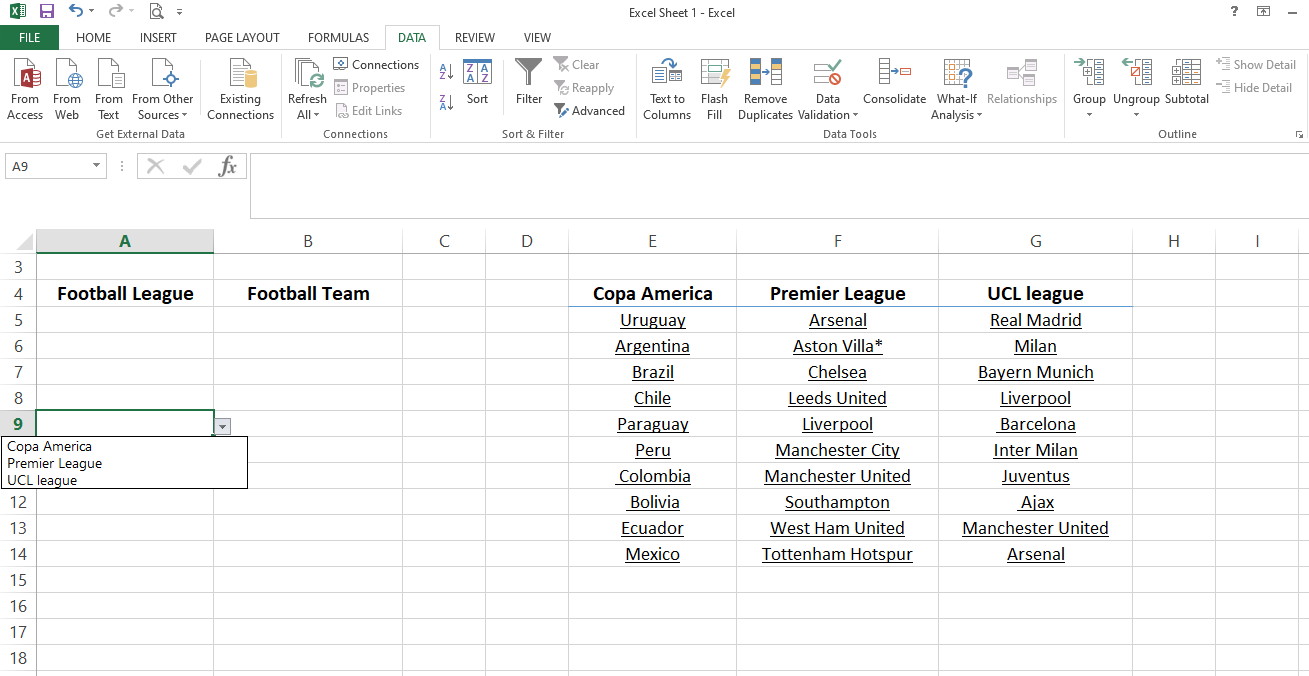
In three easy steps, you can create a simple drop-down list. Then copy and paste the formula to the rest of the cells down the row.
Creating a Dependent Drop-Down List in Excel
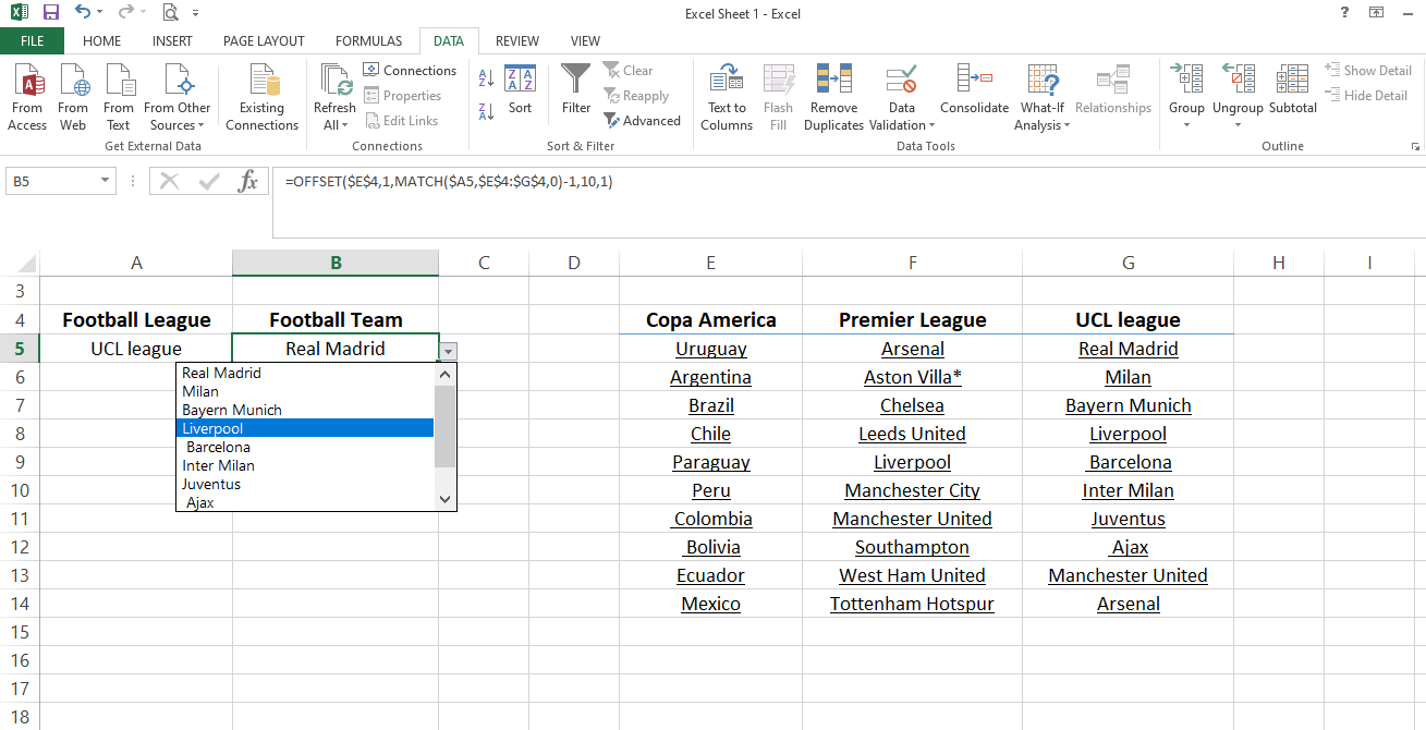
The football team's drop-down menu relies on a simple drop-down list you have just created. If you choose a specific league, then you should have the chance to select a team from the Football league drop-down menu containing only teams from that league.
Using Offset Formula to Create Drop-Down List
Let's create a formula to make sure it works perfectly before directly inserting it into the data validation box. After that, you can proceed to implement it across the whole dataset.
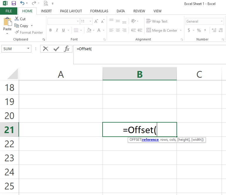
Let's take a look at the syntax of the Offset function.
The offset function has five arguments. Let's discuss them briefly here:
1. Reference: It refers to the starting point of data. The Offset function gives a range that is close to the reference point. Therefore, the reference point must be close to the dataset.
2. Rows: The rows argument refers to the number of rows you want to move down from the reference point.
3. Column: Just like rows, this argument describes the number of places you want to move across the columns of a dataset. Since the column position depends on the football league included in our simple drop-down, you may need to use the match function as a column argument.
4. Height and width: These two arguments refer to the position of cells you are currently sitting in based on the rows and columns argument selected previously. You have to count this manually, so be careful while adding the value. Also, check it twice for confirmation.
Let's implement the offset function on this dataset to understand the concept better.
Implementation of Offset Function
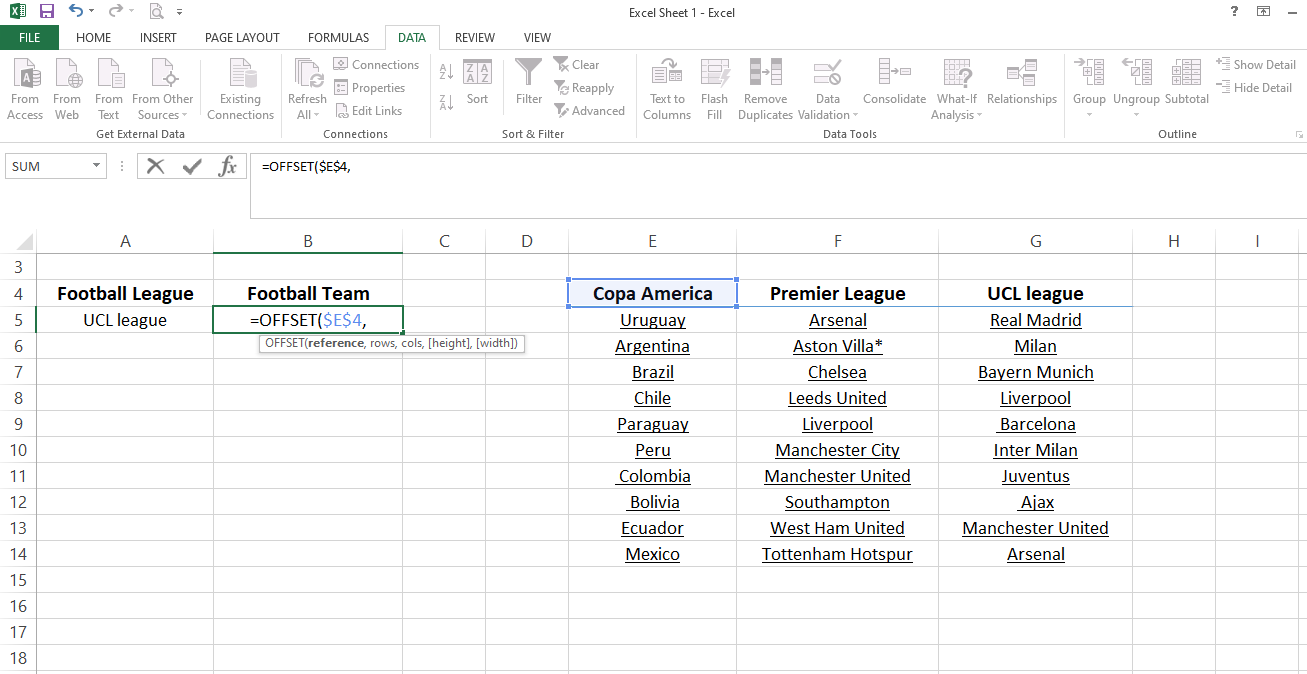
Here, cell E4 is a reference as it's the starting point of the dataset. Also, the plan is to copy the same formula to other cells down the row so you can make it an absolute cell reference by adding a $ sign.
Since the team name begins below the reference point, the row argument will be 1.
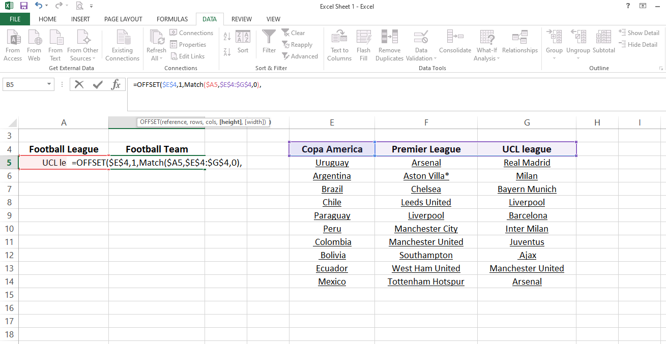
However, the height argument can change between 0, 1, and 2, and you cannot add it to each cell manually. To populate other tabs with the formula, you can use a match function that correctly assigns a column number. Let's discuss it briefly without going into too much detail.
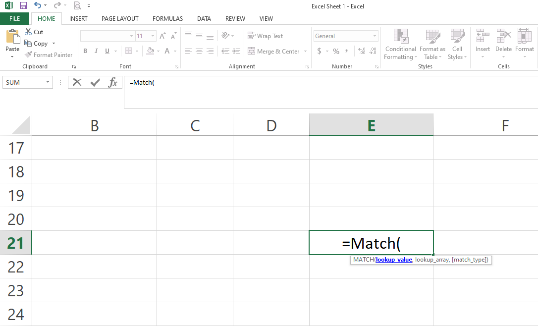
Syntax of Match Function
Lookup_value, lookup_array, and match_type are the three arguments in the match function.
In this example, the value in cell B5 is the lookup value, while the list of league names in cells E4 to G4 is the lookup array. From match_type, let's choose the exact match.
Select the whole match function and press F9 to check if it has picked the correct column position for the selected football league in the simple drop-down menu. The match function starts counting from the first column, and it considers cell E4 at position one, which is the reference point.
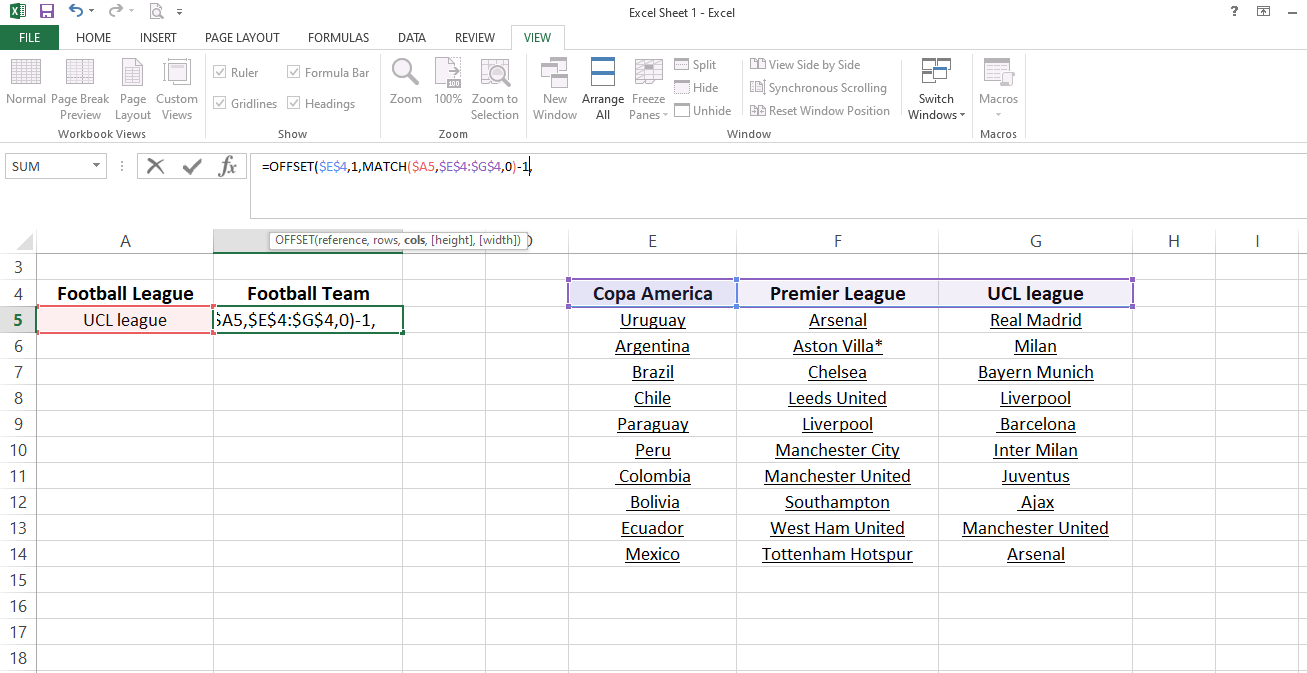
On the other hand, the offset begins counting from 0. The match function must also take the reference column at position zero to make it consistent with the offset function. To change that, subtract one from the whole formula.
Then set the height to the maximum number of values you want in the drop-down and width to one. That corresponds to the position of the row and the column in the formula.
Press enter to see if the formula has picked the right team.
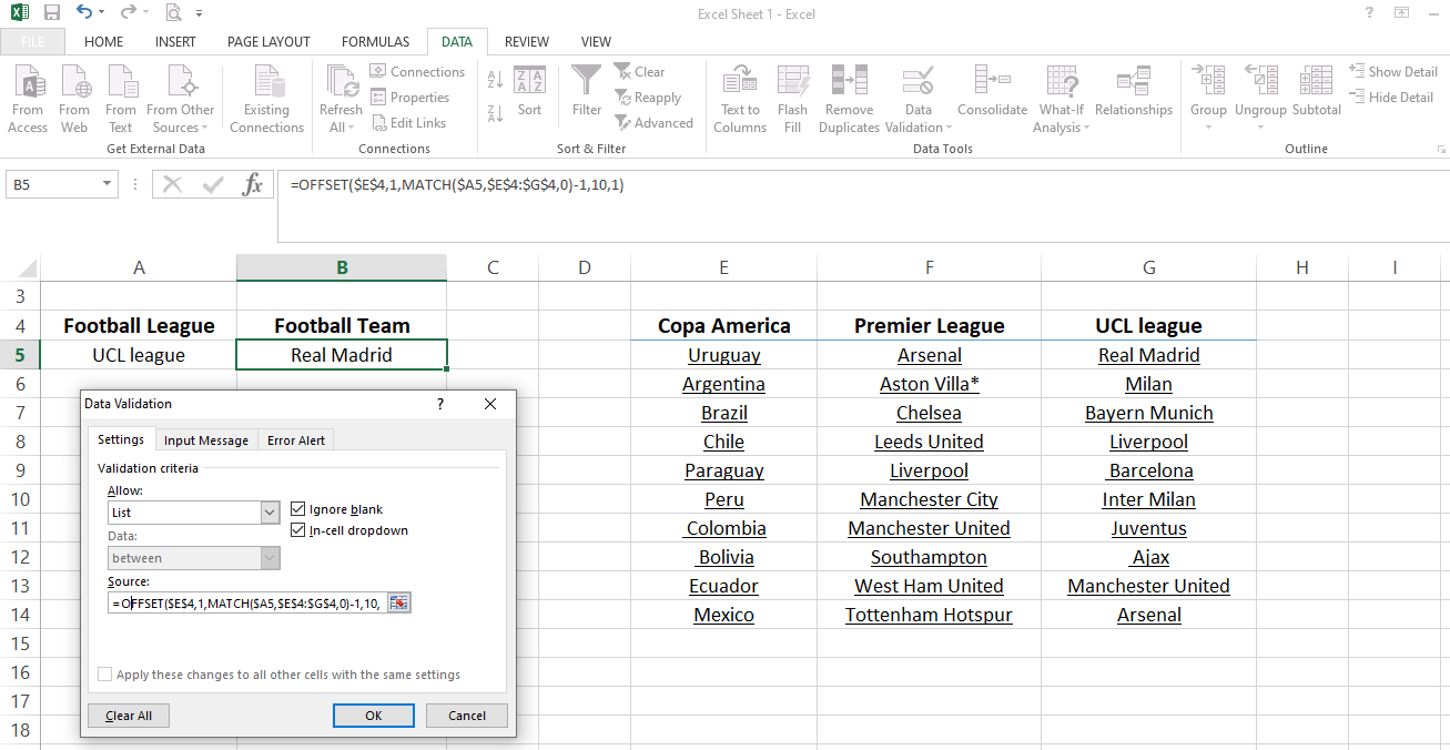
Now that the formula is ready, let's add it to data validation.
Adding Formula to Data Validation
1. By pressing CTRL + C, you can copy the formula from the selected cell.
2. Go to Data Validation.
3. Place the copied formula as the source after selecting the List as the first option.
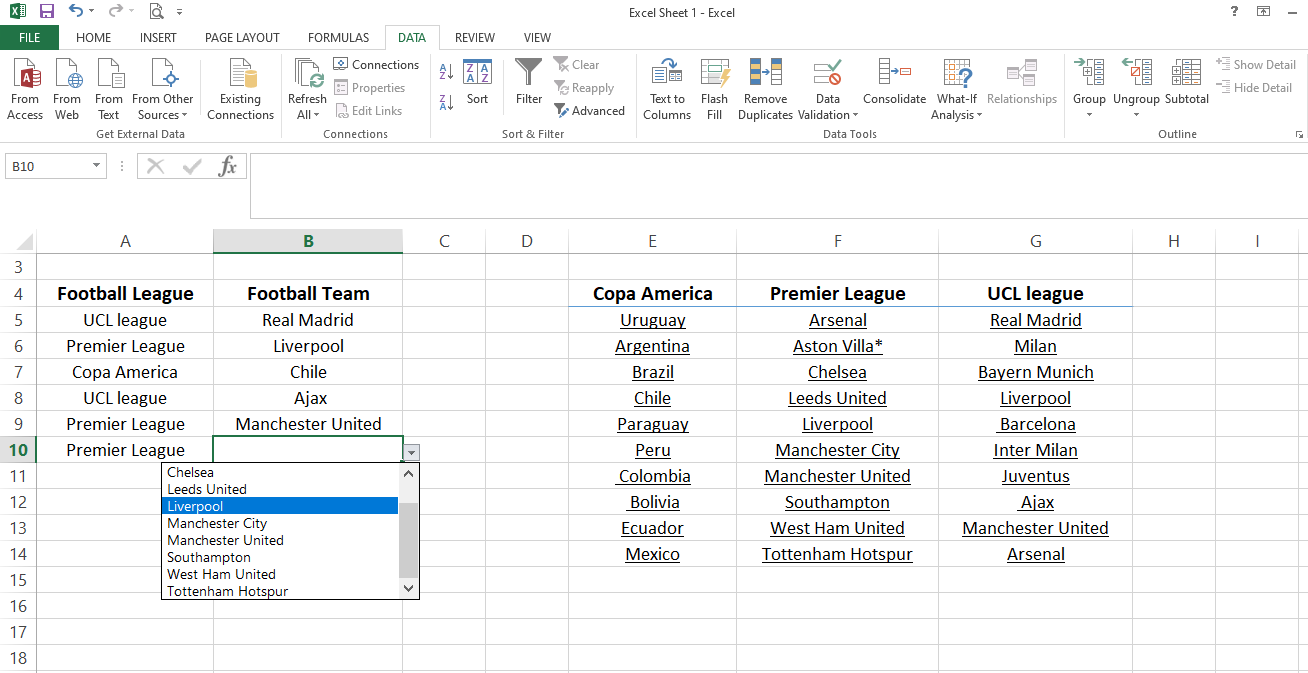
Once executed, the formula will generate multiple dependent drop-down menus for football teams.
Copy and paste the formula down the row for football teams to implement it throughout the row.
Here is how you can use the Offset formula and match function in combination to create a multiple-dependent drop-down. The offset formula may seem confusing at first, but you will get used to it after implementing it a few times.
Make Drop-Down Menus Creations Easy With Offset Formula
Many of the sheets at the workplace require you to create dropdowns. The offset formula approach is the quickest and simplest method to create the whole drop-down using just one formula.
Furthermore, it is possible to manually select cells for data validation to create dropdowns. However, manually creating dropdowns for a large dataset is time-consuming, and there is a greater chance of making mistakes. Just like Excel, you can also create a drop-down menu for Google Sheets.


