You might have been using Google Sheets for storing and visualizing numerical data for both personal and collaborative work. However, it’s not only a spreadsheet tool with many rows, columns, and formulas. You can also use it to do various cool stuff to wow your audience.

In this article, we'll introduce you to some of the best Google Sheet hacks you need to know to become a master of the platform.

1. Creating QR Codes

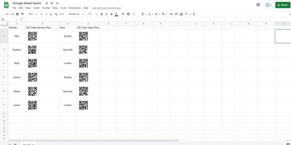
You may be in situations when you need to create QR codes to track employee attendance, student attendance, event participants, etc. You can create such codes in Google Sheets instead of relying on third-party apps or websites.

Write down the data you want in a QR code, and then use the formula snippet shown below. You’ll need to change the cell address (which in our case here is A2) to match the input data for the QR code.

        =IMAGE("https://chart.googleapis.com/chart?chs=200x200&cht=qr&chl="&A2&")")  

    

Related: Fun Things to Do With QR Codes

2. Image URLs

The image URL hack saves your time in managing images through Google Sheets. Many social media users, website developers, bloggers, etc., use spreadsheets to manage their visual assets on the internet.

Related: The Best Free Apps for Managing Your Social Accounts

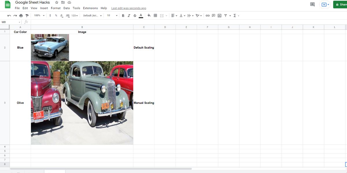
You need to manually update images if you use the conventional image insert option of Google Sheets. Instead, use a formula that automatically fetches the graphic from the internet. You can also modify the image scaling such as stretch, fit to size, etc.

Here are the steps that you can try:

1. Enter the =image(“url”) formula in the cell where you want the image.
2. Replace url in the above formula using an online link to your image.
3. Use the respective function snippet below to scale the image.
4. Press Enter to visualize the image in the cell.

        <strong>Default Image Mode:</strong> =IMAGE("https://sites.google.com/site/tepfanclub/home/jabal-jaise.jpg",1)
<strong>Manual Scaling Image Mode:</strong> =IMAGE("https://sites.google.com/site/tepfanclub/home/jabal-jaise.jpg",4,300,250)
    

3. Randomizing Names and Numbers

When choosing a name, you can make everyone happy if you draw it randomly. You may need this when selecting a team member who will work on weekends or when finding out who won a prize.

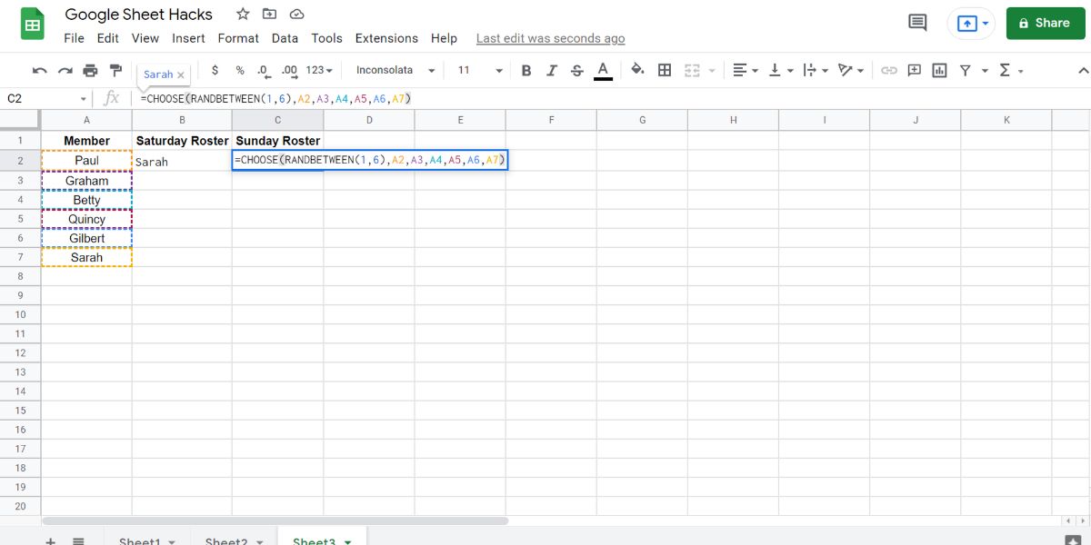
You can do such randomization easily on Google Sheets by utilizing the RANDBETWEEN formula. Try these steps yourself:

1. Note down the names of the team members in a column.
2. In the first cell of the next column, paste the function snippet mentioned below.
3. Edit the range (1,6) according to the number of names. For example, if there are 10 participants, the range will be 1,10.
4. Press Enter to get a random name.

        =CHOOSE(RANDBETWEEN(1,6),A2,A3,A4,A5,A6,A7)

    

4. Create a Drop-Down List

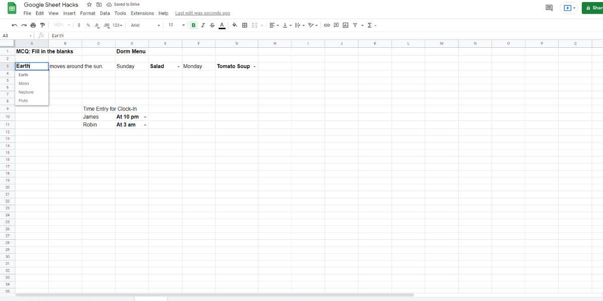
You may want to use a drop-down list to ensure team members enter specific data on the sheet. Teachers can use this method to create multiple choice questions for students. You can also create a meal menu for your home or dorm kitchen.

You can try these steps:

1. Select any cell where you want, in the drop-down list.
2. On the menu, click on Data and then choose Data validation.
3. Select a List of items as Criteria and write down the items by separating them using commas.
4. Click Save to populate the drop-down list.

5. Download Data

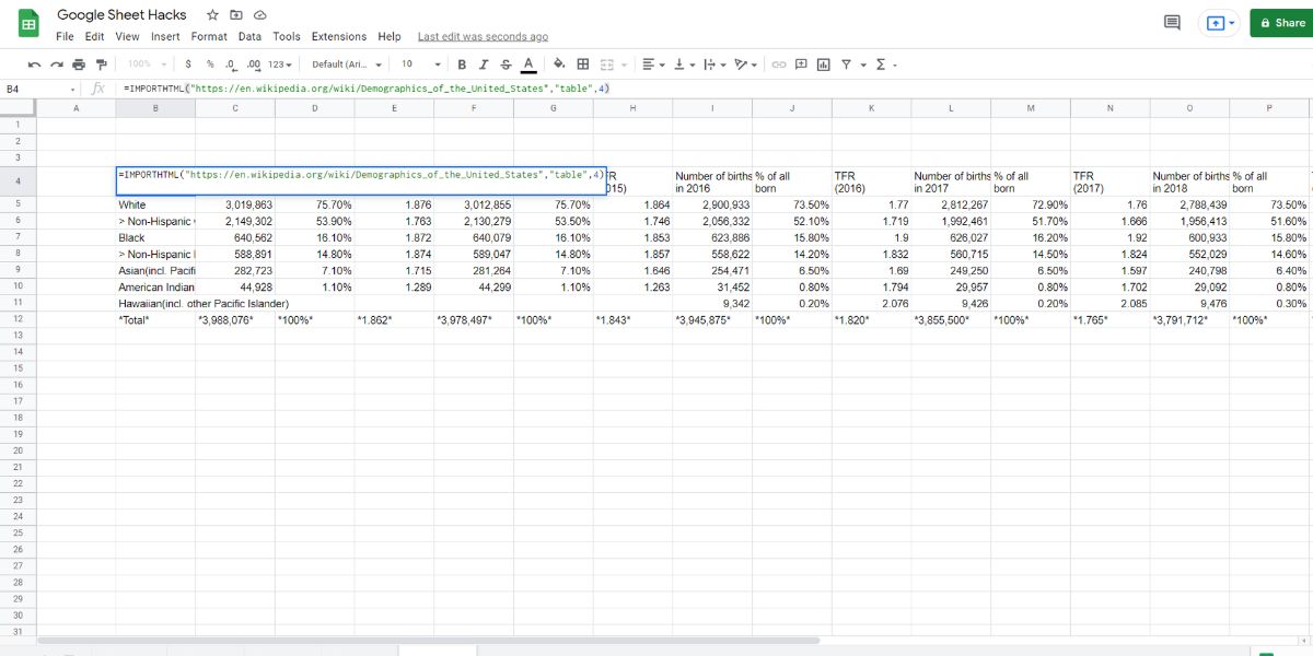
This feature lets you import/download website data into a spreadsheet. You may try the following steps to import data from any website:

1. In any cell of your worksheet, enter the below-mentioned formula snippet.
2. Replace the website address in the parenthesis with your target website.
3. Hit Enter to load data into your worksheet.

        =IMPORTHTML("https://en.wikipedia.org/wiki/Demographics_of_the_United_States","table",4)
    

6. Self-Checking Assessments

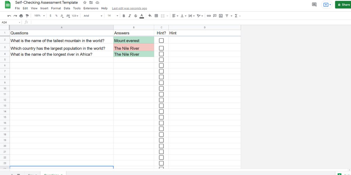
You can utilize the Conditional formation option of Google Sheets to make self-checking question papers. It’s helpful if you’re preparing for an upcoming exam. You can write down the questions and answers in their respective sheets.

Then, hide the sheet that contains answers. On the question sheet, write down your answer to find out how's your exam preparation is. You can use this ready-to-use template to get started.

7. CLEAN and TRIM Functions

Google Sheets cleans and trims data on its own. However, you may find unprintable characters or unnecessary spacing between texts or formulas. It often happens with shared spreadsheets.

You can use the CLEAN formula to delete all unprintable characters from data instead of manually correcting them one by one. You can use the TRIM function to remove unwanted spaces between names, email addresses, or formulas.

8. Split Data

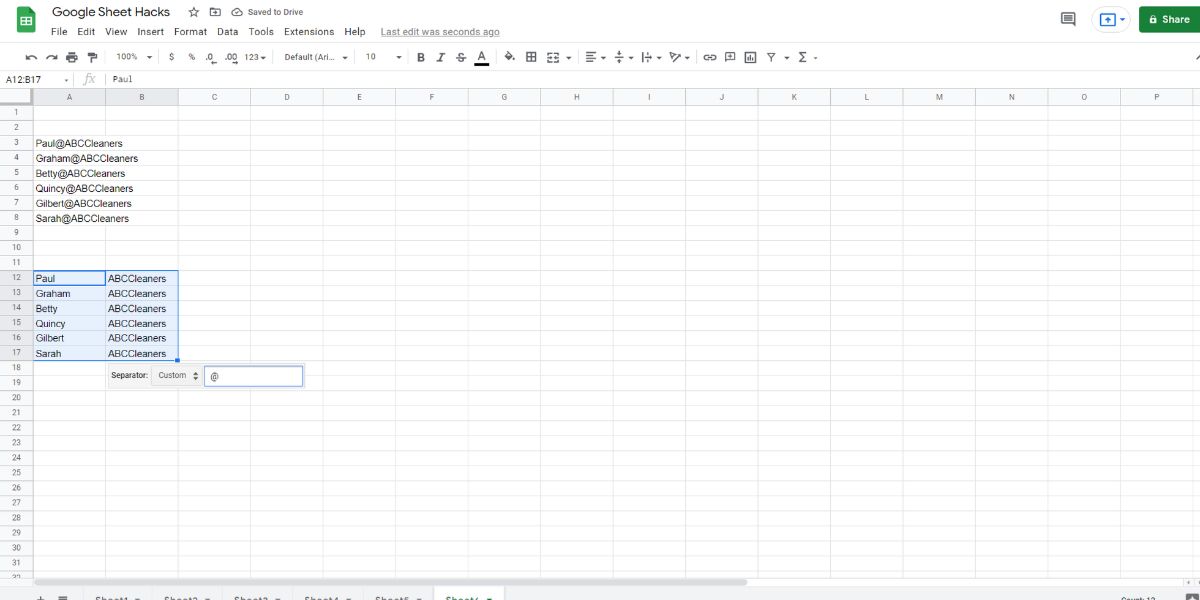
In many instances, you may need to split texts into two different columns from one cell. You’ll end up losing the entire workday if you start doing that manually for each cell, especially for spreadsheets with thousands of data.

Utilizing this function is easy if you follow these steps:

1. Select the entire data that you want to split into two columns.
2. Click on Data in the menu bar and then select Split text to columns.
3. You can either choose any of the displayed separators or select a custom character.
4. You’ll see split texts as soon as you choose a valid separator.

9. Visualize All Keyboard Shortcuts

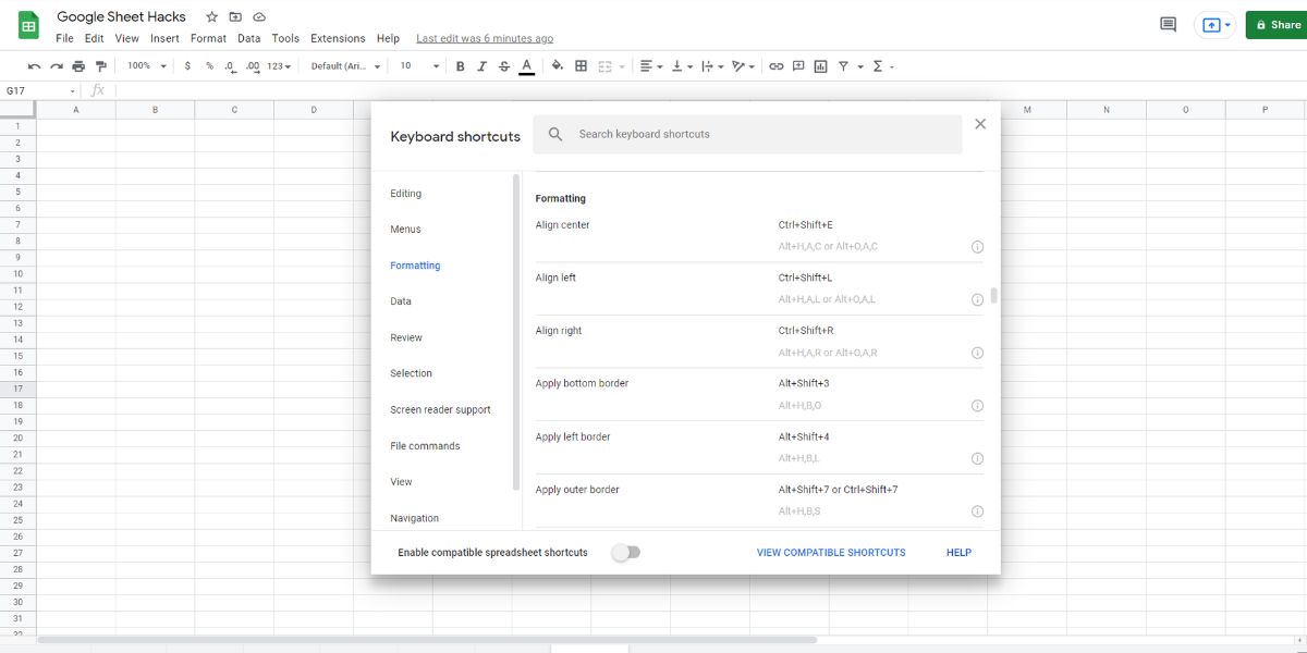
You should start using the keyboard shortcuts if you want to increase your productivity on Google Sheets. However, remembering all keyboard shortcuts like clearing cell formatting, hiding rows, adding comments, etc., are not easy. With this trick, you can bring all the keyboard shortcuts in front of you while you’re working on Google Sheets.

Press Ctrl + / on a Windows computer or Command + / on a macOS computer to bring up the Google Sheets keyboard shortcut list. Whenever you forget a shortcut, visualize them on your screen to use shortcuts instead of a mouse. You'll soon memorize all vital keyboard shortcuts by repeating this practice.

10. Find Related Data

It’s a time taking task to look for data for a report that you’re creating. Instead, you can use any data finder add-ons for Google Sheets. There are many data finder add-ons, and some of them are also free to use.

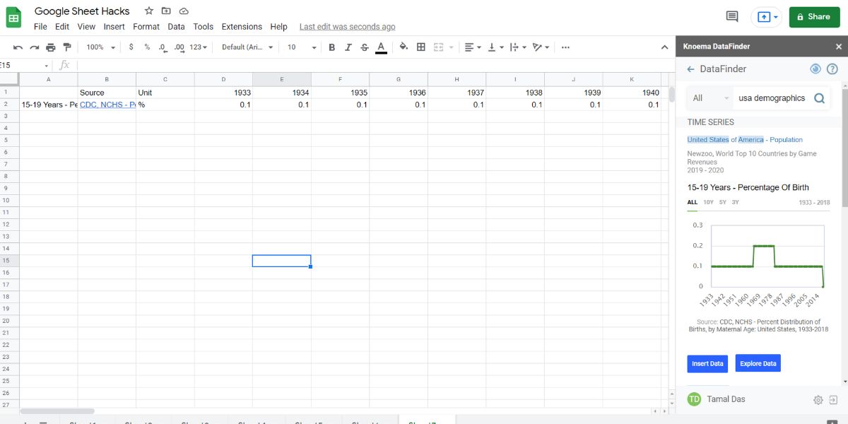
For example, you can install the Knoema DataFinder add-on in your Google Sheets. You can bookmark your own data to the add-on.

While you’re making any report, simply open the add-on and fetch bookmarked data. You can also search the internet for your report-related data and insert that in your report quickly.

Get Things Done With Google Sheets

The above-mentioned quick hacks of Google Sheets will surely help you to solve day-to-day challenges in school, office, or home.

These are also quite easy to learn than other complex tricks of Google Sheets. Moreover, the above tips help you visualize your data by saving time and adding innovation to your report.