Google Sheets is a great online spreadsheet app for sorting, calculating, and analyzing data. The program has numerous features, which is why learning how to use Google Sheets can seem daunting to people who are not familiar with it. However, once you get the hang of it, using it is a breeze.

The following guide teaches beginners different ways to format data in Google Sheets. We’ll help you learn how to group together rows, split columns, hide gridlines, and more.

1. Group Rows in Google Sheets

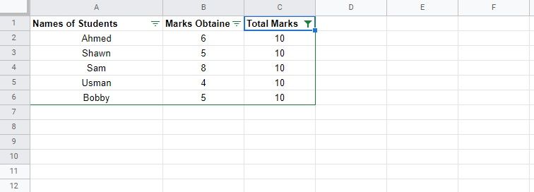
Consider you have the following marks sheet:

To group rows of the marks sheet, follow the steps below:

1. Select the rows you want to group. In this example, let’s select rows 2 to 6.
2. Go to the Google Sheets Menu Bar at the top.
3. Click View, then go to Group and select Group rows 2 - 6.

Another method to group rows is as follows:

1. Select the rows you want to group together.
2. Right-click the mouse or mouse pad.
3. Go to View more row actions.
4. Select Group rows 2 - 6.

After grouping the rows by any of the above-mentioned methods, your rows will look like this:

As you can see, there’s a minus sign above the grouped rows. You can easily collapse (or expand) the grouped rows from here.

2. Delete Every Other Row in Google Sheets

Consider the data in the image below:

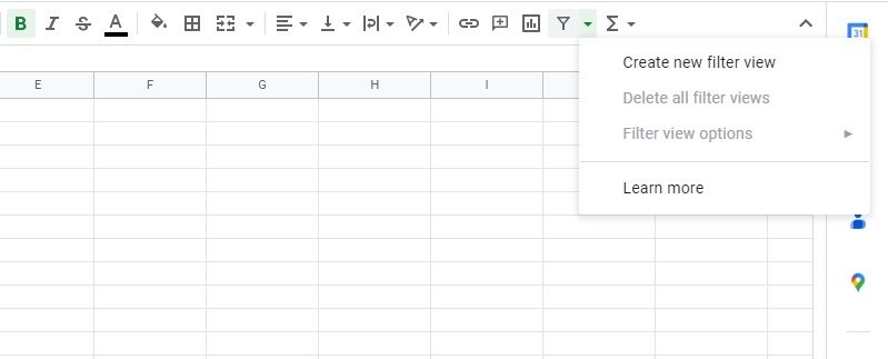
Follow the steps below to delete every other row using the Google Sheets filter function:

1. Select the first row (i.e., A1:C1).
2. Go to Create a Filter icon in the Menu Bar and select Create new filter view. You’ll see that the entire first row has filter icons.

   

3. Go to the filter icon and select Filter by condition.
4. In the Filter by condition, select Custom formula is.

   

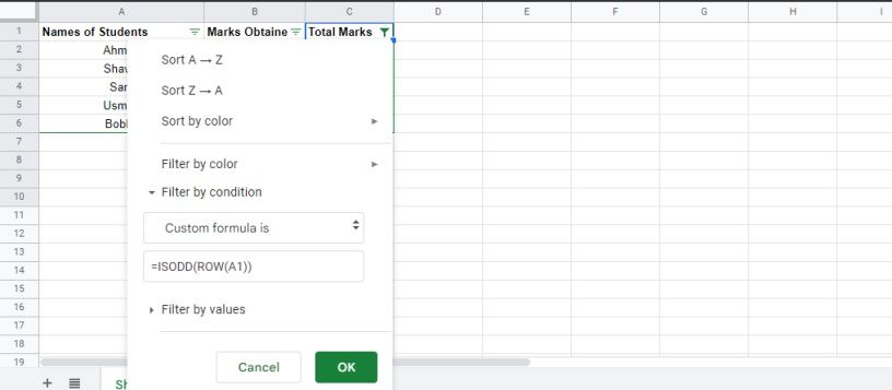
5. Enter the following formula in the blank text box:

           =ISODD(ROW(A1))
       

6. Select OK. You’ll see that every other row in the marks sheet has been deleted.

   

3. Move Rows & Columns in Google Sheets

When working in Google Sheets, you’ll often need to move columns to better format your spreadsheet. If you’re not sure how to do that, follow any of the methods below:

Using Google Sheets' Native Tool

To move a column using the Google Sheets native tool, follow the steps below:

1. Select the column you want to move.
2. Go to Edit in the Menu Bar.
3. Click Move.
4. Select Column left or Column right if you want the column to move left or right, respectively.

To move a row using Google Sheets' native tool, follow the steps below:

1. Select the row you want to move.
2. Go to Edit in the Menu Bar.
3. Click Move.
4. Select Row up or Row down if you want to move the row up or down, respectively.

Using the Cut/Paste Option

1. Select the data in the column (or row) you want to move.
2. Right-click your mouse or mouse pad and select Cut.
3. Go to the column (or row) you want to move the data to.
4. Right-click your mouse or mouse pad and select Paste.

Using the Drag/Drop Option

The simplest way of moving rows or columns in Google Sheets is by selecting the entire row or column you want to move, and then dragging and dropping it at the desired spot.

4. Combine and Split Columns in Google Sheets

Sometimes you need to combine two separate columns together while formatting in Google Sheets. As a beginner, you might not know how to do it, but it’s pretty simple:

1. Select the columns you need to combine.
2. Click the drop-down arrow next to the Select merge type icon and select Merge horizontally.

   

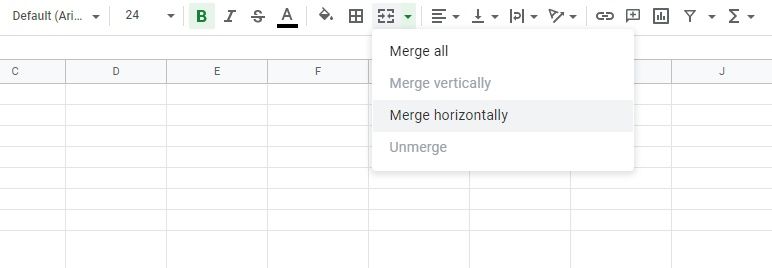
3. A pop-up will appear, prompting you that only the top-leftmost value will remain in the merged cell.

   

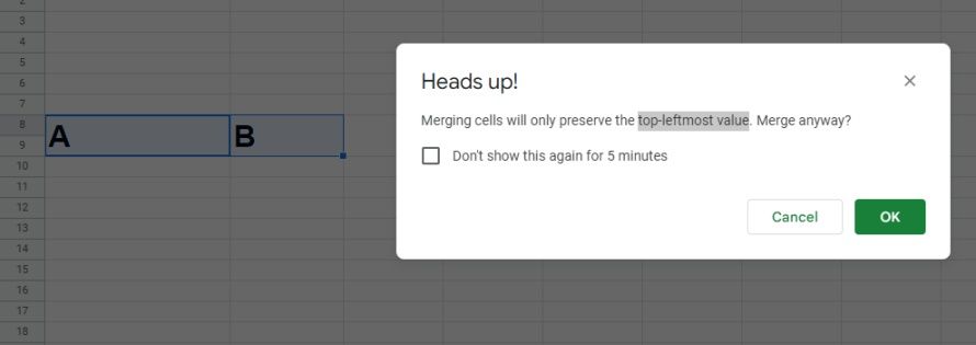
4. Click OK and the two columns will combine (or merge) into one.

To unmerge this cell, go to the Select merge type icon and select Unmerge. But what if you want to split the text inside a column into two or more columns?

Suppose we have a set of student names and want to split them into their first and last names. You can do that with the help of the Split text to columns function by following the steps below:

1. Select the column you want to split.

   

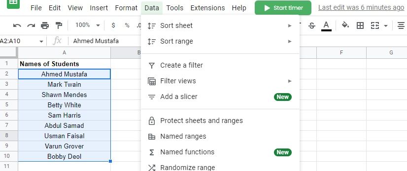
2. Click Data (in the Menu Bar) and select Split text to columns.
3. You’ll see that a Separator box appears just below the selected data. Set the separator to Space.

   

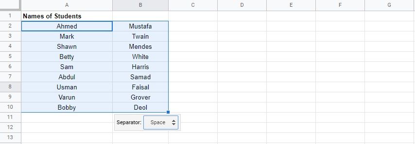
In the separator, we select Space because, in our case, the text (names) we want to split into columns are separated by a space. If the names were separated by a comma, period, or semicolon, we’d select that as the separator.

5. Hide Gridlines in Google Sheets

Gridlines are the foundation of any spreadsheet (Excel or Google Sheets). They help separate the data in each cell, making the data collection or calculation much easier.

However, once you’re done with your spreadsheet and want to print out the results, removing the gridlines is often a good idea to make the printout less cluttered and easy on the eyes. Just as you can hide gridlines in Microsoft Excel, you can do so in Google Sheets as follows:

1. Go to View in the Menu Bar.
2. Select Show.
3. Click Gridlines to uncheck it.

You might want to remove the gridlines of a specific section in your sheet. In that case, select the area where you want to remove the gridlines and follow the above-mentioned steps. If you want to retain the gridlines in the original sheet and remove them in the printout, you can do that by following the steps below:

1. Press CTRL + P to open up the Print settings page.
2. Under Formatting in the right panel of the Print settings page, uncheck Show gridlines.
3. Select Next to see the preview (you’ll see that it has no gridlines).
4. Click Print.

6. Hide or Delete Unused Rows & Columns in Google Sheets

When you’re done working on your sheet and don’t need to add any information, you can hide all the unused cells in the sheet. This gives it a cleaner look and increases emphasis on only the used cells.

Here’s how you can hide unused cells in Google Sheets:

1. Select all the unused columns by selecting the first unused column (Column D in our case), then pressing CTRL + Shift + right arrow key.
2. Now that you have selected columns D to Z, right-click the highlighted area and click Hide columns D - Z.
3. You can also delete the columns by clicking Delete columns D - Z.

To hide all unused rows, follow the steps below:

1. Select all the unused rows by selecting the first unused row (Row 11 in our case), then pressing CTRL + Shift + down arrow key.
2. Now that you have selected rows 11 to 1000, right-click the highlighted area and click Hide rows 11 - 1000.
3. You can also delete the rows by clicking Delete rows 11 - 1000.

Make Your Spreadsheets Visually Pleasing

By now, you’ve probably become a master at playing with rows and columns in Google Sheets. You’ve learned how to hide or delete unused rows/columns, combine or split columns, different ways to move rows and columns, and learned other formatting operations in Google Sheets.

You can use these formatting operations to make your spreadsheets visually pleasing and easier to read. But learning is far from over. There’s a lot more you can do with Google Sheets to format your spreadsheets better. Do you know how to format cell values in Google Sheets? Maybe it’s time to take the next step.