You can fit a lot of data into an Excel sheet. With thousands upon thousands of rows and columns, it can get pretty unwieldy.
One small feature that makes it easier to manage all of that data is the ability to freeze rows and columns. This means that no matter where you scroll in the spreadsheet, those rows or columns always stay visible.
Along with the freeze feature in Excel is a lock option. While it may sound like these two features could do the same thing, they actually serve different purposes. To avoid confusion, we'll explain the difference and then how to lock rows, columns, and cells in Excel as well.
Freeze Versus Lock in Excel
As we briefly mentioned above, if you want a row or column to be visible no matter where you scroll in your Excel sheet, this requires the freeze feature.
You would use the lock feature to prevent changes to the content of a cell. As examples, you might lock a cell or range that contains formulas, lists, or similar types of data that you don't want changed.
So if someone asks you how to lock a row in Excel, they likely mean to ask how to freeze a row in Excel.
How to Freeze the First Column or Top Row in Excel
More spreadsheets than not contain column or row headers. So freezing a column or row containing headers make is much easier to manage your data, especially when you have a lot of it.
With this method, you're going to have to choose to freeze either the first column or first row. Unfortunately, you can't do both.
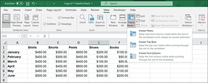
- Open your Excel spreadsheet and go to the View tab.
- Click the Freeze Panes button.
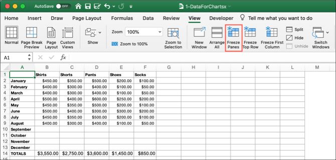
- To freeze the first column, click Freeze First Column in the dropdown menu. To freeze the top row, click Freeze Top Row.
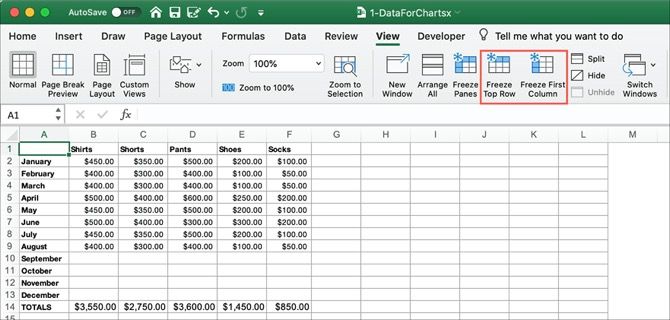
In Excel on Mac, you have separate buttons on the View tab for each option. So just click Freeze First Column or Freeze Top Row.
How to Freeze Columns and Rows in Excel
You may want to freeze more than just the first column or row in Excel. For instance, maybe you want to freeze the first three columns or rows.
- Open your Excel spreadsheet and go to the View tab.
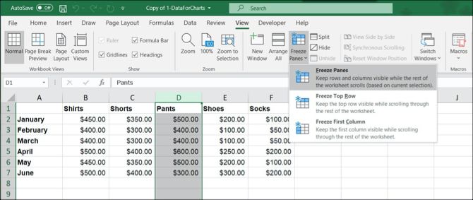
- Select the last column or row in the group you want to freeze. For example, if you want to freeze columns A through C, select column D. Or if you want to freeze rows 1 through 4, select row 5.
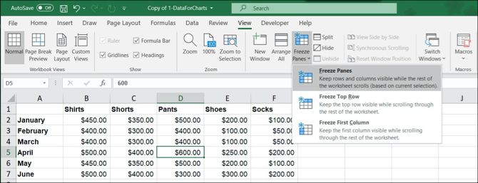
- Click the Freeze Panes button and then the Freeze Panes option in the dropdown menu.
In Excel on Mac, this is also its own button on the View tab. So select the column or row and click Freeze Panes.
How to Freeze Panes in Excel
If you would prefer to freeze a combination of rows and columns, referred to as a pane, it's possible but slightly trickier.
- Open your Excel spreadsheet and go to the View tab.
- Select the cell directly below the row you want to freeze and the cell to the right of the column you want to freeze. For example, if you want to freeze columns A through C and rows 1 to 4, you would select cell D5.
- Click the Freeze Panes button and again, click the Freeze Panes option in the dropdown menu.
How to Unfreeze Columns, Rows, or Panes in Excel
It's just as simple to unfreeze columns, rows, and panes in Excel as it is to freeze them.
- Open your Excel spreadsheet and go to the View tab.
- Click the Freeze Panes button.
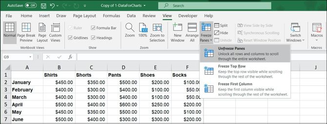
- Select Unfreeze Panes in the dropdown menu.
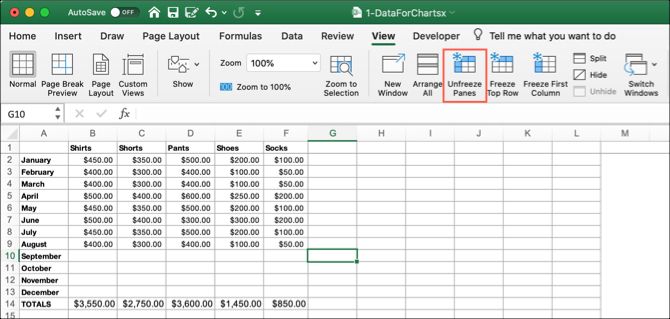
In Excel on Mac, as you may have already guessed, this too is its own button. Head to the View tab and click Unfreeze Panes.
How to Lock Columns, Rows, or Cells in Excel
Locking rows, columns, or cells in Excel involves two steps. First, you'll lock the cell(s) and then you'll protect the sheet. Note that cells in Excel are locked by default, but we'll show you how to double-check that for the two-step process.
This process can stop rows from being deleted in Excel.
Lock the Cell(s)
- Select the column, row, cell, or group that you want to lock.
- Open the Format Cells dialog box by clicking the Alignment group on the Home tab or by right-clicking the cell(s) and picking Format Cells.
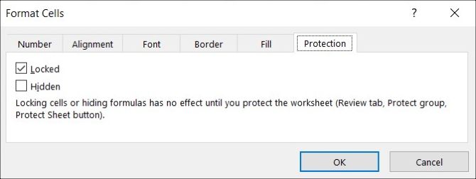
- Choose the Protection tab.
- Make sure the box for Locked is checked and click OK.
Protect the Sheet
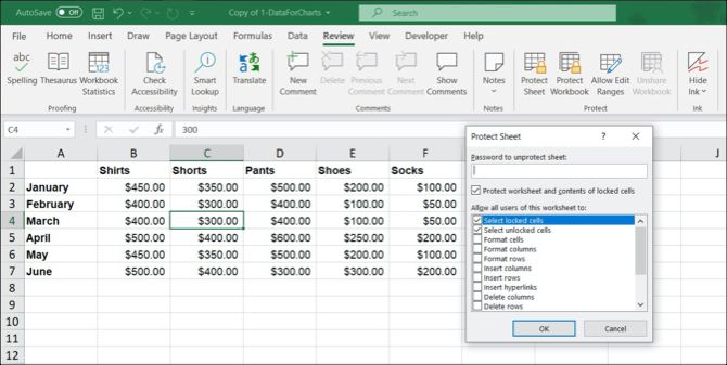
- Go to the Review tab and in the Protect group click Protect Sheet.
- In the pop-up window, you'll see a list of optional items that you can check or uncheck as part of the protection. Make sure that the first box is checked for Protect worksheet and contents of locked cells. If you want to allow other users to select the cells you lock, but not change them, you can check the box for Select locked cells.
- Enter a password for the sheet in the box at the top and click OK. On Windows, you'll need to verify your password and click OK once more. On Mac, the password and verification are on the same screen.
Unprotect the Sheet
To remove protection from an Excel spreadsheet, go to the Review tab, click Unprotect Sheet, and enter the password.
If you're interested in the Protect Workbook button that you see in the ribbon, check out our tutorial on how to use that to protect your Excel file.
What's important to note when you lock cells and protect a sheet is that as we explained earlier, all cells in an Excel sheet are locked by default. So unless you specifically unlock cells, all cells will be locked.
Lock Only Certain Cells
If you only want specific cells to be locked, you'll start by unlocking them all and then only locking the ones you want.
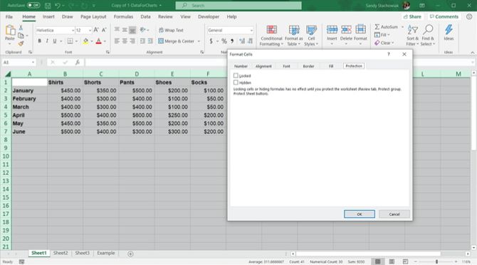
- Click the Select All button (triangle) on the top left of the sheet. You'll see your entire spreadsheet become highlighted.
- Open the Format Cells dialog box by clicking the Alignment group on the Home tab or by right-clicking the cell(s) and picking Format Cells.
- Choose the Protection tab.
- Uncheck the box for Locked and click OK.
Once you do this, all cells in the spreadsheet will be unlocked. Now you can follow the two-step process above to Lock the Cell(s) and Protect the Sheet.
Freeze for Easy Viewing, Lock to Prevent Changes
Freezing rows and columns along with locking cells can both help in different situations. Whether you want to see a large amount of data more easily or make sure unwanted changes don't occur, Microsoft Excel gives you the features you need.
And for doing more with your Excel spreadsheets, take a look at tips for working with worksheet tabs or how to manage columns in Excel.

