Many apps can create checklists, but do you need yet another app? For example, if you're already using spreadsheets, you can easily make a checklist in Microsoft Excel.

Even if you don't want to use it as a simple to-do list app, a checklist is an excellent way to track what you still need to do in your spreadsheet directly in the spreadsheet itself.

Let's see how to create a checklist in Excel in five minutes or less.

How to Make a Checklist in Excel

We'll show you how to create an Excel checklist with checkboxes you can tick off as you complete the items. It will indicate when you've checked off all the items so you can tell at a glance.

Here are the simple steps we'll outline below:

1. Enable the Developer Tab.
2. Enter the checklist items into your spreadsheet.
3. Add the checkboxes and advanced formatting.

1. Enable the Developer Tab

You must enable the Developer tab on the ribbon to create a checklist. To do this, right-click on the ribbon and select Customize the Ribbon.

In the list of Main Tabs on the right side of the Excel Options dialog box, check the Developer box and click OK.

2. Enter the Checklist Items Into Your Spreadsheet

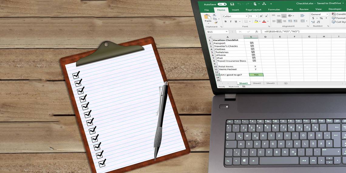
Enter your to-do list, one item per cell. In our example, we have a cell with the Total Items, and one with the total Items Packed, or how many items are checked off on our list.

The Am I good to go? cell will be red with NO if all the items are not checked off.

Once you check off all the items, the Am I good to go? cell turns green and will read YES.

Click the Developer tab. Then, click Insert in the Controls section and click the Check Box (Form Control).

3. Add the Checkboxes

Select the cell in which you want to insert the checkbox. You'll see that there's text to the right of the checkbox. We only want the text box, not the text. While the checkbox control is selected, highlight the text next to the checkbox, and delete it.

The checkbox control does not automatically resize once you've deleted the text. If you want to resize it, right-click on the cell to select the checkbox and then left-click on it (to make the context menu disappear). It will be selected with circles at the corners (as shown above).

Drag one of the circles on the right side towards the checkbox to resize the outline to just the size of the checkbox. Then, you can move the checkbox to the center of the cell with the four-headed cursor.

We want to copy that checkbox to the rest of our to-do list items.

To select the cell containing the checkbox, select any cell around it without a checkbox. Then, use one of the arrow keys on your keyboard to move to the cell with the checkbox.

To copy the checkbox to the other cells, move your cursor over the bottom-right corner of the selected cell with the checkbox until it turns into a plus sign. Make sure the cursor is NOT a hand. That will check the box.

Drag the plus sign down over the cells into which you want to copy the checkbox and release the mouse button. The checkbox is copied to all those cells.

Advanced Checklist Formatting

Depending on what you want to use your checklist for, you can add additional formatting elements to validate your list and display its status.

Create a True/False Column

For this step, we need to use the column to the right of the checkboxes to store the TRUE and FALSE values for the checkboxes. That allows us to use those values to test whether all the boxes are checked.

Right-click on the first checkbox (not the cell with the checkbox) and select Format Control.

On the Control tab on the Format Object dialog box, click the cell selection button on the right side of the Cell link box.

Select the cell to the right of the checkbox cell. An absolute reference to the selected cell is inserted in the Cell link box on the compact version of the Format Control dialog box.

Click the cell selection button again to expand the dialog box. Finally, click OK on the dialog box to close it.

Repeat the procedure for each checkbox in your list.

Enter Total Items and Calculate Items Checked

Next, enter the total number of checkboxes in your list into the cell to the right of the Total Items cell.

Let's use a special function that calculates how many checkboxes have been checked.

Enter the following text into the cell to the right of the cell labeled Items Packed (or whatever you called it) and press Enter.

        =COUNTIF(C2:C9,TRUE)
    

This counts the number of cells in the C column (from cell C2 through C9) that have the value TRUE.

In your sheet, you can replace "C2:C9" with the column letter and row numbers corresponding to the column to the right of your checkboxes.

Hide the True/False Column

We don't need the column with the TRUE and FALSE values showing, so let's hide it. First, click on the lettered column heading to select the whole column. Then, right-click on the column heading and select Hide.

The lettered column headings now skip C, but a double line indicates a hidden column.

Check If All Checkboxes Are Checked

We'll use the IF function for Am I good to go? (or whatever you call it) to see if all the checkboxes are checked. Select the cell to the right of Am I good to go? and enter the following text.

        =IF(B11=B12,"YES","NO")
    

This means that if the number in cell B10 is equal to the number calculated from the checked boxes in B11, YES will be automatically entered in the cell. Otherwise, NO will be entered.

Apply Conditional Formatting

You can also color code the cell based on whether the values in cells B10 and B11 are equal. This is called Conditional Formatting.

Let's see how to turn the cell red if not all the checkboxes are checked and green if they are. See our article about Conditional Formatting for information on how to create rules.

Select the cell next to "Am I good to go?". It's B14 in this example spreadsheet.

Create a rule for this cell with the Conditional Formatting Rules Manager dialog box. Go to Home > Conditional Formatting > New Rules. Then, select the Use a formula to determine which cells to format rule.

Enter the following text in the Format values where this formula is true box.

Replace B11 and B12 with the cell references for your Total Items and Items Packed (or whatever you named these cells) values if they're not the same. (See our guide to the Excel name box if you need more info on that.)

        =$B11<>$B12
    

Then, click Format and select a red Fill color and click OK.

Create another new rule of the same type, but enter the following text in the Format values where this formula is true box. Again, replace the cell references to match your checklist.

        =$B11=$B12
    

Then, click Format and select a green Fill color and click OK.

On the Conditional Formatting Rules Manager dialog box, enter an absolute reference for the cell you want to color green or red in the Applies to box.

Enter the same cell reference for both rules. In our example, we entered =$B$13.

Click OK.

The Am I good to go? cell in the B column turns green and reads YES when all the checkboxes are checked. If you uncheck any item, it will turn red and read NO.

Excel Checklist Complete? Check!

You can create a checklist in Excel easily enough. But it is just one type of list. You can also make dropdown lists in Excel with your custom items.

Do you also have information that you often use, like department names and people's names? Try this method to create custom Excel lists for recurring data you always need.